Week 1- Mixing Tee

Simulation of turbulent and thermal mixing in T-junctions using Ansys fluent

Objective-

To simulate and analyze the turbulent and thermal mixing of fluids of different temperature in a T-junction of a pipe of different lengths and see the effectiveness of mixing of the fluids.

Introduction-

Mixing Tees utilizes a specifically engineered internal geometry to efficiently mix two fluid streams into one combined stream. Mixing tees are widely used in the petrochemical, HVAC industry etc. in which two fluid streams with different physical and/or chemical properties mix together.

Turbulent mixing of fluid of different temperature in T-junction geometries has also become of significant importance in the field of nuclear reactor safety.

Hot air flowing in the main pipe is mixed with cold air flowing through a tee. The standard deviation of temperature is computed to quantify the degree of mixing. The average velocity and average temperature are also computed at the end of the pipe.

For this, we have created two versions of the tee model of which one of them is longer than the other to see the effect of the length on mixing.

It is set up as a steady-state simulation to compare the mixing effectiveness when hot inlet temperature is 36^oC & the cold inlet is at 19^oC.

1. Case 1
• Short mixing tee with a hot inlet velocity of 3m/s.
• Momentum ratio of 2, 4.
2. Case 2
• Long mixing tee with a hot inlet velocity of 3m/s.
• Momentum ratio of 2, 4.

Momentum ratio is defined as the ratio of velocity at the cold inlet to the velocity at the hot inlet.

Procedure-

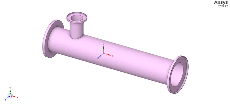
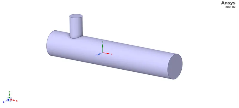
1. CAD cleanup/Pre-processing (SpaceClaim) - The CAD model is imported into the SpaceClaim to extract the flow volume field from the model. The CAD model and the extracted volume is shown below-

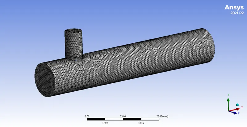
2. Meshing- Mesh generation and boundary name is done in this part to specify the inlet, outlet and the wall of the model for simulation. Mesh element size is 0.002m.

3. Setup-

For this inputs or boundary conditions, we have to specify the inlet and outlet velocity which we already have assigned in the model. By default ansys fluent takes fluid material as air and solid material as aluminum. So, we don’t have to change the material here.

Now, we will initialize the model after selecting the solver type and viscous model, for making contours and plots of average temperature, velocity and standard deviation in each iteration. For the initialization we are choosing hybrid model. Also, here we have selected K-omega SST model for the viscous model.

Results-

Case 1

1. Short mixing tee with a hot inlet velocity of 3m/s.
2. Momentum ratio of 2, i.e., cold inlet velocity is 6m/s.

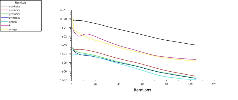
Residual Plot-

Average temperature plot-

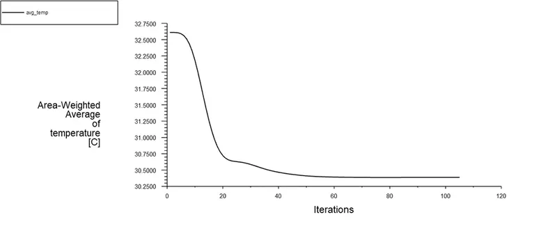
Here, you can see the solution converged after 105 iterations and the average temperature is 30.47^o Celsius.

Standard deviation plot-

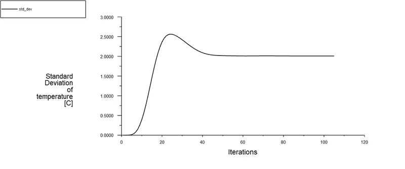
Here, you can see the standard deviation of temperature is 2.1 after solution converged. The standard deviation tells how much the temperatures at the outlet differs from the mean temperature and this case does not good results at the outlet.

Temperature contour –

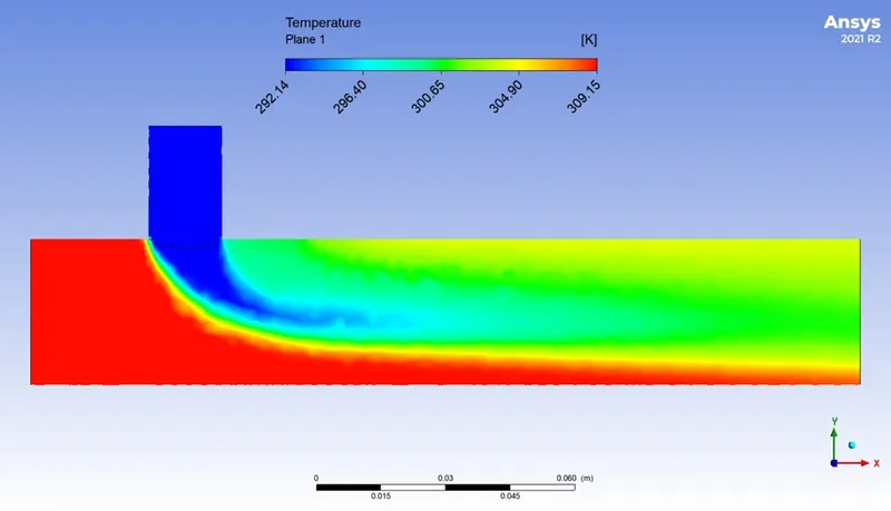
Here, you can see how the cold and hot fluid fluids mix in the short tee at less velocity of cold fluid.

Velocity contour-

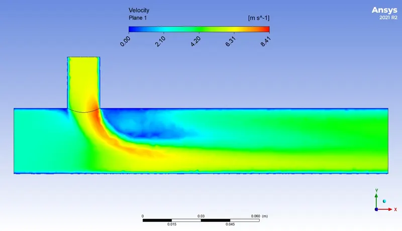
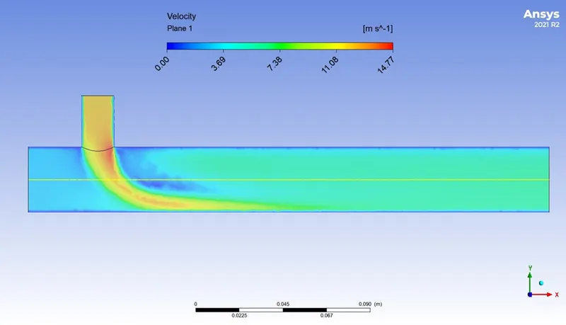
The above contour shows the magnitudes of velocity at different parts of the short tee and the results of the mixture of both the fluids.

Temperature and velocity vector contour-

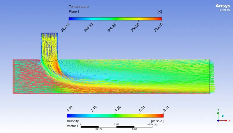
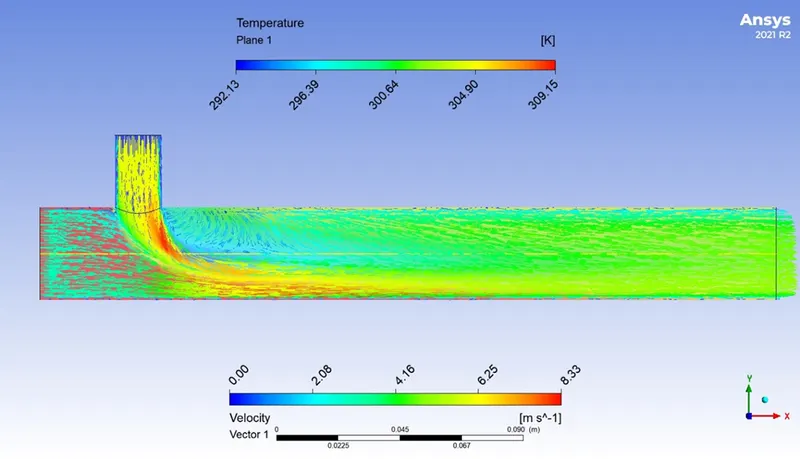
The above contour shows the temperature as base of the plane and above are the arrows or vectors of velocity showing the flow of the fluids in the short tee.

Case 2

1. Short mixing tee with a hot inlet velocity of 3m/s.
2. Momentum ratio of 4, i.e., cold inlet velocity is 12m/s.

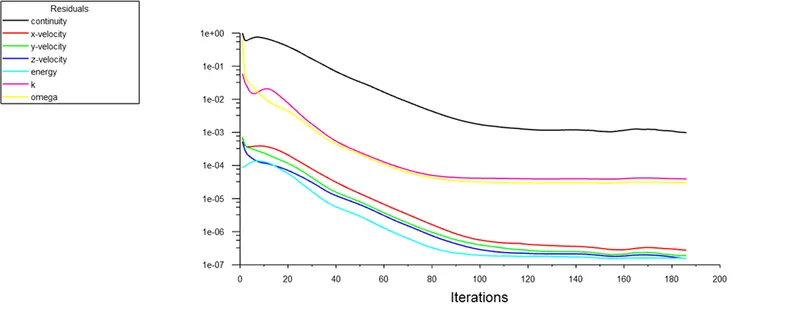
Residual Plot-

Average temperature plot-

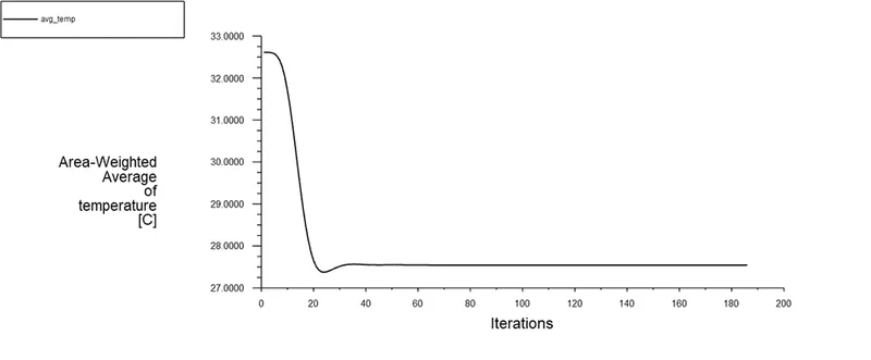
Here, you can see the solution converged after 185 iterations and the average temperature is 27.55^o Celsius.

Standard deviation plot-

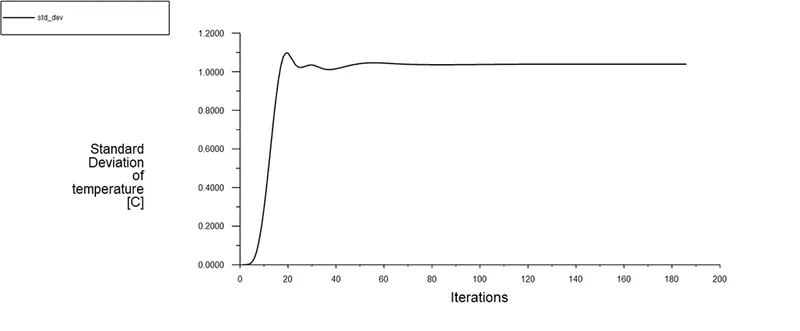
Here, you can see the value of standard deviations is almost equal to 1 which is very good result which tells the temperatures of fluid at the outlet is very close to mean temperature.

Temperature contour-

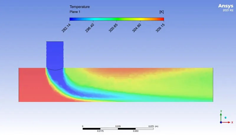
Velocity contour-

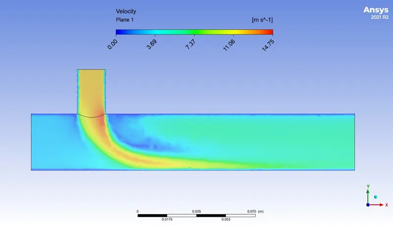
Case 3

1. Long mixing tee with a hot inlet velocity of 3m/s.
2. Momentum ratio of 2, i.e., cold inlet velocity is 6m/s.

Residual plot-

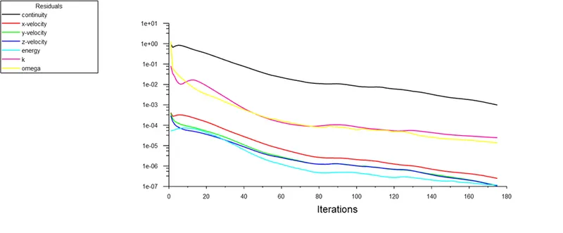
Temperature plot-

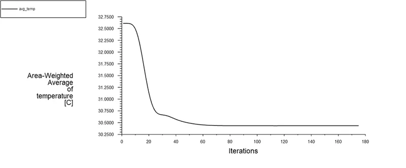
Here, you can see the solver converges after 175 iterations and the average temperature is 30.46^o Celsius.

Standard deviation plot-

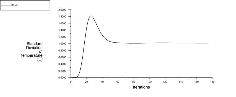
Here, you can see the standard deviation is almost equal to 1 which tells us that there is good mixture of the two fluids in the long tee.

Temperature contour-

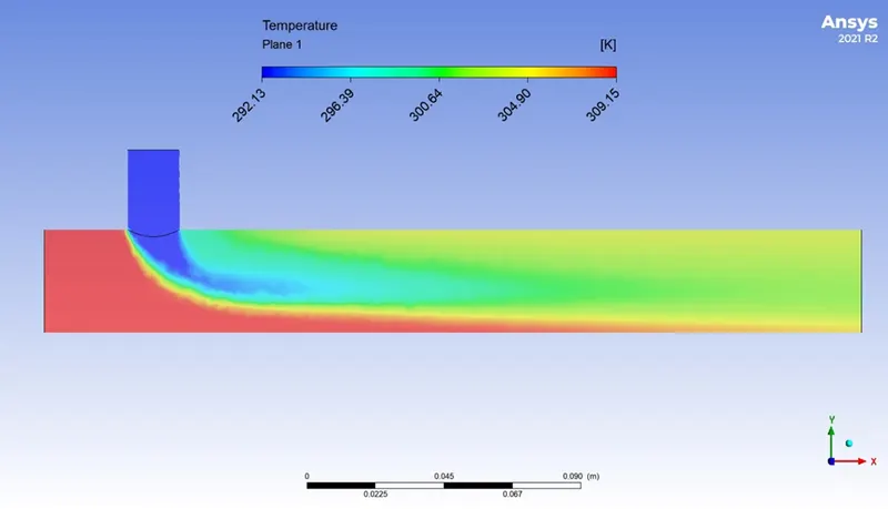
Velocity contour-

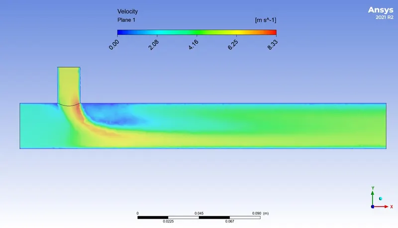
Temperature velocity vector contour-

Case 4

1. Long mixing tee with a hot inlet velocity of 3m/s.
2. Momentum ratio of 4, i.e., cold inlet velocity is 12m/s.

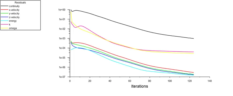
Residual plot-

Temperature plot-

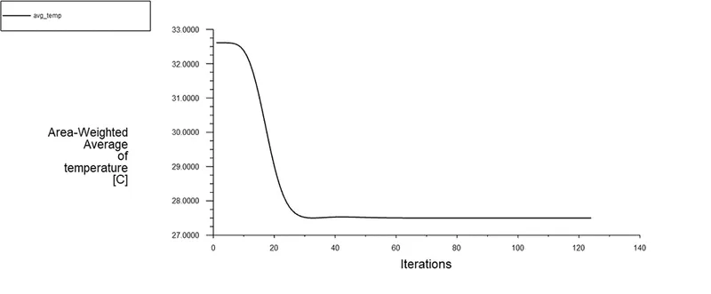
Here, you can see the solver converges after 125 iterations and the average temperature is 27.48^o Celsius.

Standard deviation plot-

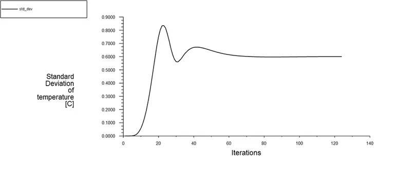
Here, you can see the standard deviation is about 0.6 which tells that the most average temperatures of the fluid at the outlet is not close to the mean temperature, i.e., the mixture of the fluids did not happen very efficiently.

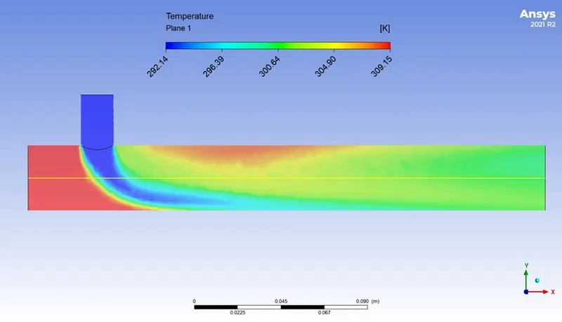
Temperature contour-

Velocity contour-

Conclusion-

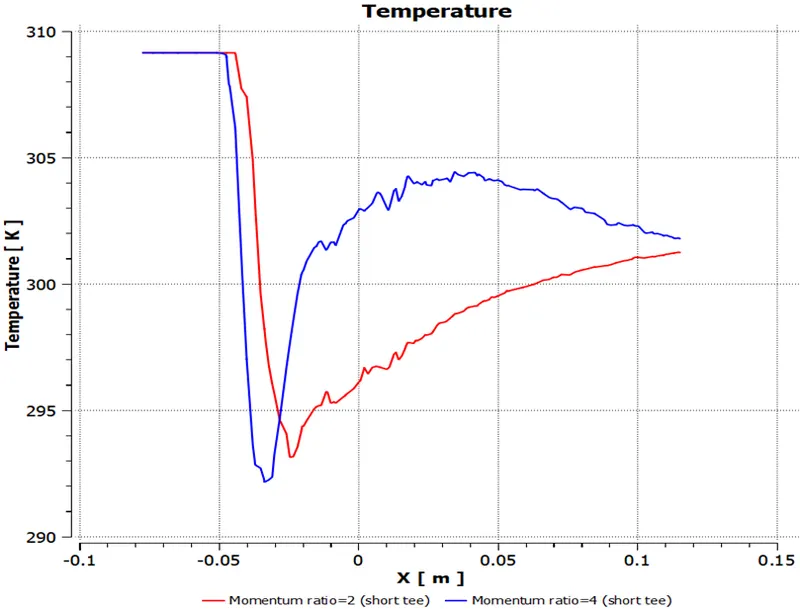
The above chart shows the average temperature comparison between the different momentum ratios along the length of the short tee pipe.

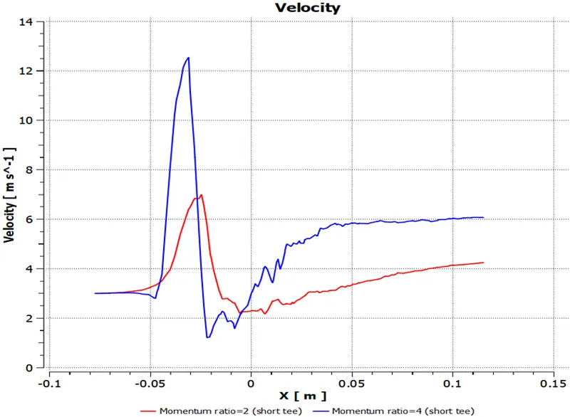
The above chart shows the velocity comparison between the different momentum ratios along the length of the short tee pipe.

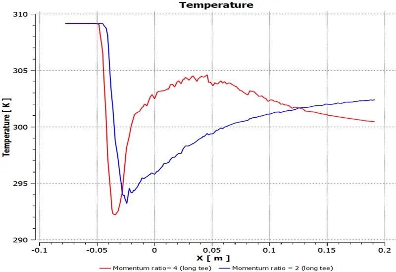
The above chart shows the average temperature comparison between the different momentum ratios along the length of the long tee pipe.

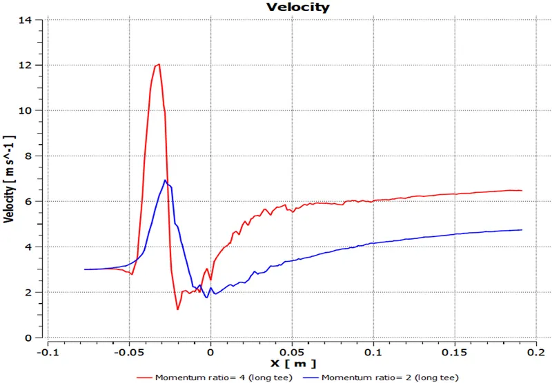
The above chart shows the velocity comparison between the different momentum ratios along the length of the long tee pipe.

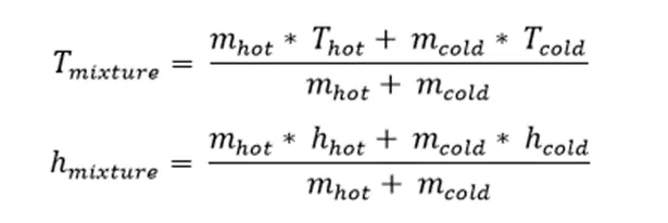
The temperature of the fluid at the outlet of the pipe is compared with the help of the numerical formula which is shown below-

Parameters	Outlet temperature (C)		Percentage Error (%)
	Analysis	Numerical
Case1: Short Tee
Momentum ratio = 2	30.47	30.32	0.47
Momentum ratio = 4	27.55	27.49	0.12
Case2: Long Tee
Momentum ratio = 2	30.46	30.32	0.44
Momentum ratio = 4	27.48	27.49	0.02

As you can see from the above calculations, momentum ratio greatly affects the outlet average temperature in both the cases. Also, due to increase in velocity the time for mixing of the fluids is lesser due to which the temperature is higher when the momentum ratio is 4.

Also, due to increased velocity the numerical and analytical temperatures at the outlet has very less error as compared to the lower momentum ratio cases.