Week 4 - CHT Analysis on Exhaust port

Conjugate Heat Transfer Analysis on Exhaust port

Objective-

To perform steady state conjugate heat transfer (CHT) analysis on exhaust port using air as the fluid.

Introduction-

The Conjugate Heat Transfer (CHT) analysis type allows for the simulation of heat transfer between solid and fluid domains by exchanging thermal energy at the interfaces between them. Conjugate heat transfer analysis describes the heat transfer between a body and a fluid flowing over or inside it as a result of interaction between two objects. At the matching interface, the details are provided for temperature distribution and heat flux along the interface, eliminating the need of calculating the heat transfer coefficient.

Conjugate heat transfer (CHT) analysis can accurately predict heat transfer by simultaneous solving all the relevant solid and flow field heat transfer processes, for example: conduction through solids, free and forced convection in the gases/fluids and thermal radiation.

The CHT approach has an advantage over FE thermal analyses in that wall heat transfer coefficients and their local variations on surfaces are directly calculated within the model rather than based on simplified empirical calculations. The CHT approach therefore has benefits for those applications where heat transfer is either non-uniform or difficult to calculate empirically.

Typical applications of this analysis type exist as, but are not limited to, the simulation of heat exchangers, cooling of electronic equipment, and general-purpose cooling and heating systems. CHT in recent years has significantly improved the cooling performance of electronic equipment such as the design of heat sinks and the design of heat exchangers for the waste treatment plant. One such application of CHT is the exhaust port system.

Procedure-

Below is the model of the exhaust port-

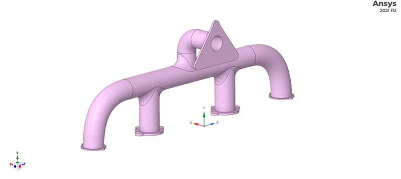
Now, in space claim we have to extract the volume to show the fluid flow volume inside the exhaust port. After the volume extraction we have to use share topology tool since we have to transfer information between the volume extracted and the outer solid exhaust port in the correct way.

Below is the image after volume extraction and using share topology tool-

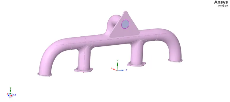
Meshing-

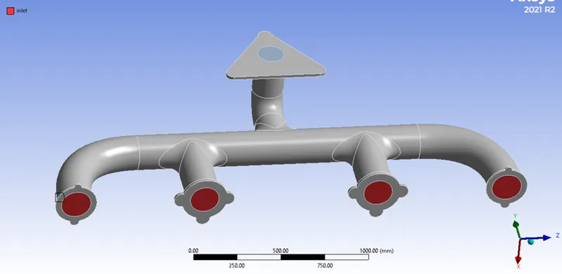
Initially generate mesh using element size of 100mm. Now, before adding inflation layer name the surfaces. Below surfaces in the red are named as inlet-

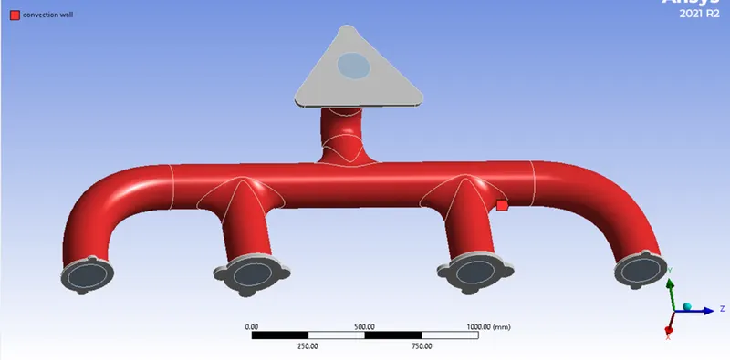
In the image below, the outer surfaces of the exhaust port is named as convection wall-

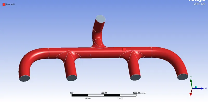
In the image below, the outer surfaces of the extracted fluid volume is named as fluid wall -

Now, we have to add the inflation layer and for that we have the required inputs below-

Free stream inlet velocity- 5m/s

Density of fluid – 1.019 kg/m3

Dynamic viscosity of fluid (µ) – 0.000026 Ns/m2

Characteristic length (D) – 0.16 m (diameter of pipe)

Desired Y+ value – 5 (based on K-omega model)

Thus, Reynold’s no = 31538.46, first layer height = 0.6mm, and boundary layer thickness by using Re and L came out be 7.946mm.

Below image shows the model after meshing with inflation layer body sizing the fluid volume with element size = 15mm (case1) -

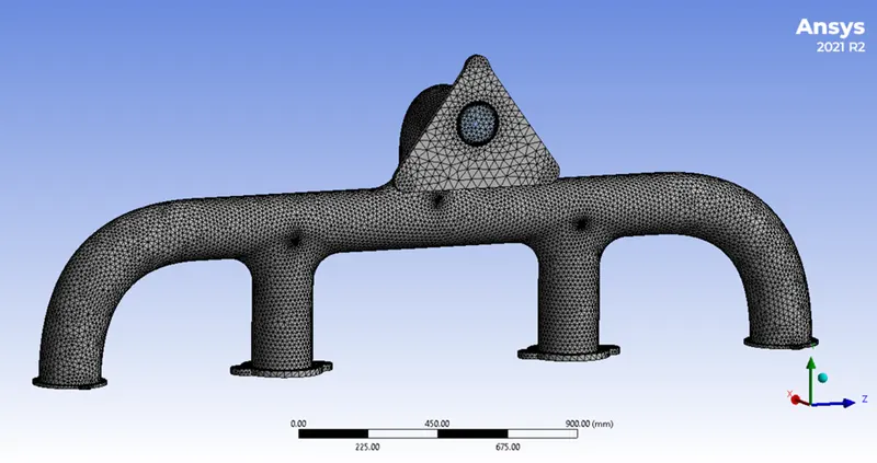
For case 2, the element size is 10mm.

Pre-Processing and Solver Setting:

We are solving using steady state and K-omega SST model as viscous model.

Under the cell zone conditions check if the exhaust port is solid and if the fluid region is automatically selected as fluid.

Under the boundary condition, input velocity at the inlet = 5m/s and temperature at inlet = 700K.

Under the convection tab for convection wall change the heat transfer coefficient to 20 Watt/ (m2K).

For creating heat transfer coefficient report -

Report definition>surface report>area weighted average>under field variable select wall fluxes and heat transfer coefficient then select surfaces as fluid wall.

Now initialize the problem using hybrid initialization and start the solution for 500 iteration.

Results-

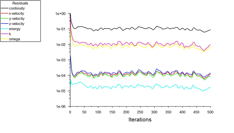
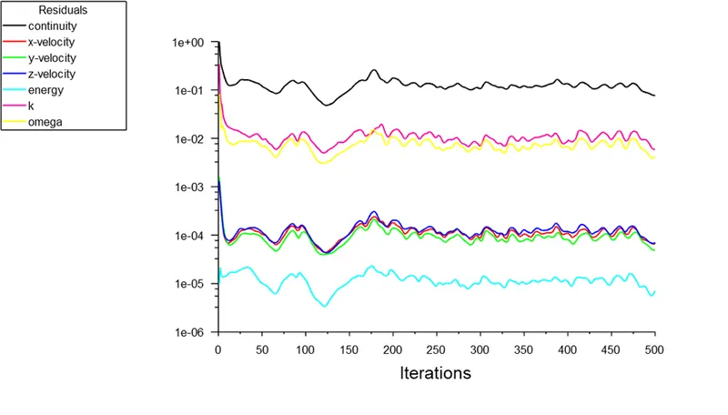
Below image shows the plot of scaled residuals for case 1 and 2-

Below image shows the plot of average heat transfer coefficient for case 1 and 2-

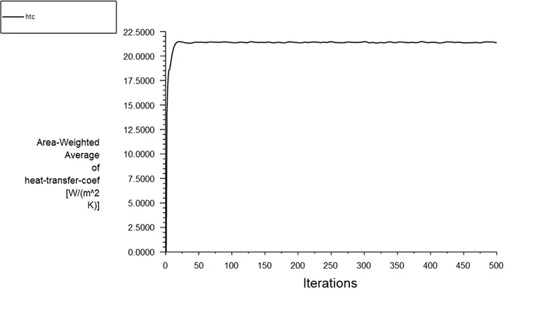
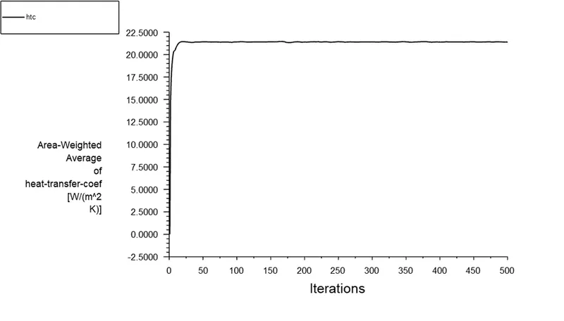
As you can see in the above plots of heat transfer coefficient, the solution converged after 50 iterations only.

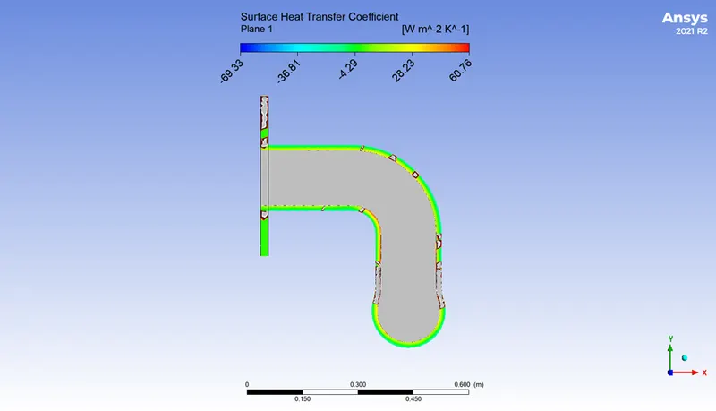
Below image shows the contour of surface heat transfer coefficient at the outlet pipe-

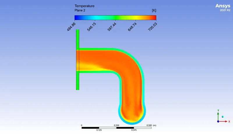
Below image shows the contour plot of temperature at the outlet pipe-

Below image shows the contour plot of velocity at the outlet pipe-

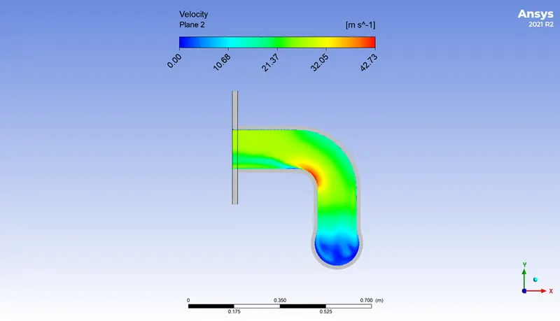
You can see that the velocity at the outlet is more than the inlet since there are 4 inlets and only one outlet.

Below image shows the contour plot of velocity vector at the outlet pipe-

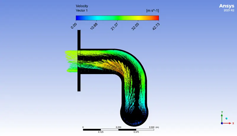
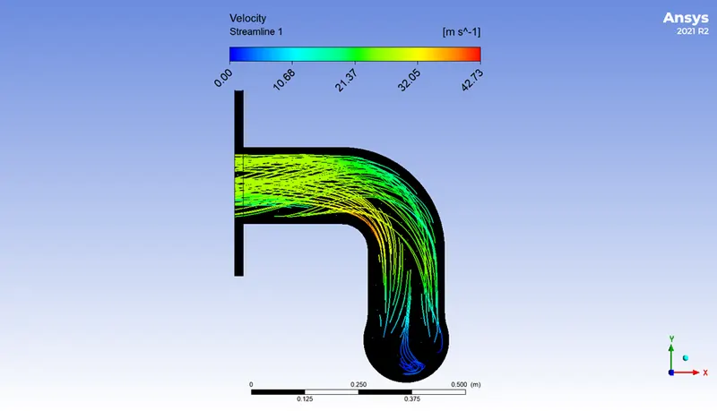
Below image shows the contour plot of velocity streamline at the outlet pipe-

Analytical solution-

The Reynolds number for the given flow is 31538.46 which suggests that the flow is turbulent in nature, the Dittus Bolter heat transfer coefficient relation can be used to determine the Nusselt number which is described mathematically as follows

Nu = 0.023 * Re^0.8 * Pr^0.3

where Prandl number (Pr) = (µ*Cp)/K = (0.000026*1026)/0.03931 = 0.68

Thus, Nu = 81.38

Now, heat transfer coefficient = (K * Nu)/D = 19.99 W/m²K

Conclusion-

Sr. no.	Element size	No. of elements	Heat transfer coefficient (W/m2K)	Analytical heat transfer coefficient (W/m2K)	Error percentage
1.	15mm	492189	21.386	19.99	6.52
2.	10mm	1185839	21.342		6.33

As you can see from the above table, the error in the numerical and analytical heat transfer coefficient is found to be between 6-7%.

The value of the heat transfer coefficient for the second and final mesh refinement are close to each other and we can omit decrease in element size to save computational time.