Explicit and Implicit Analysis
Objective:
To study and understand the implicit and explicit analysis method and use them to solve a simple numerical problem.
Implicit vs Explicit:
Explicit methods are those in which the information at time step n+1 can be obtained in terms of previous time steps and there is no dependence on the current time step. Implicit methods are those where the information at the time step n+1 is dependent on previous time levels and the current i.e. n+1. Implicit analysis requires a numerical solver to invert the stiffness matrix once or even several times over the course of a load/time step. This matrix inversion is an expensive operation, especially for large models. Explicit doesn't require this step. In the nonlinear implicit analysis, the solution of each step requires a series of trial solutions (iterations) to establish equilibrium within a certain tolerance. In the explicit analysis, no iteration is required as the nodal accelerations are solved directly. The time step in the explicit analysis must be less than the Courant time step (the time it takes a sound wave to travel across an element). Implicit transient analysis has no inherent limit on the size of the time step. As such, implicit time steps are generally several orders of magnitude larger than explicit time steps.
| Explicit | Implicit | |
| Stability | Conditional stability governed by CFL condition. Time steps are smaller of the order of 1E-06 sec for a mesh size of 5mm. | Unconditionally stable. Usually, large time steps of the order of 1E-03 sec are used. |
| Computational speed / Cost | Very fast as there is no matrix inversion. Mass matrix is lumped or diagonal. | Equally fast as one can take larger time steps. |
| Numerical scheme | Central difference method |
1. Newmark beta integration scheme. |
| Handling nonlinearity | Linear to highly nonlinear problems can be efficiently handled. Best suited for highly nonlinear problems such as crash analysis. | Linear to moderate nonlinear problems can be solved. Most suitable applications are static to vibration problems such as frequency response ad quasi-static simulations. |
Now let's solve a simple problem given below using both implicit and explicit methods.
`f(u) = u^3+9u^2+4u` -------------------------------------(1)
`k(u) = (df)/(du) = 3u^2+18u+4` ------------------------------(2)
where,
- u= displacement
- f= internal force
- K = stiffness
- F= external force
- ∆u = incremental displacements
- ∆F = incremental external load.
Explicit method:
Step 1:
`u_0 = 0`,
`k(u_0) = 3(u_0)^2+18(u_0)+4 = 4`,
`∆F = 1`,
`∆u1 = (∆F)/(k(u_0)) = 1/4 = 0.25`,
`u_1 = u_0+∆u_1= 0.25`,
Step 2:
`u_1= 0.25`,
`k(u_1)= 3(0.25)^2+18(0.25)+4 = 8.6875`,
`∆F = 1`,
`∆u_1 = (∆F)/(k(u_1)) = 1/8.6875 = 0.1151`,
`u_2 = u_1+∆u_2 = 0.3651`
Step 3:
`u_2= 0.3651`,
`k(u_2)= 3(0.3651)^2+18(0.3651)+4 = 10.9716`,
`∆F = 1`,
`∆u_2 = (∆F)/(k(u_2)) = 1/10.9716 = 0.09114`
`u_3 = u_2+∆u_3 = 0.46`
Finally, from the three steps, the following results are obtained.
`F_(ext) = ∆F+∆F+∆F = 3`
`f_(i n t) = (0.46)^3+9(0.46^2)+4(0.46) = 3.79`
It is evident from the results that external and internal forces are not in equilibrium because `F_(ext) != f_(i n t)`. The table below summarizes the main results for the explicit analysis.
| Step i | `∆F_i` | `k(u_i)` | `∆u_i` | `u_i` | `(F_(ext))_i` | `(f_(i n t))_i` | `f_(i n t) - F_(ext) = R` |
| 1 | 1 | 4 | 0.25 | 0.25 | 1 | 1.578125 | 0.578125 |
| 2 | 1 | 8.6875 | 0.1151079137 | 0.3651079137 | 2 | 2.70883602 | 0.7088360204 |
| 3 | 1 | 10.97185381 | 0.09114230076 | 0.4562502144 | 3 | 3.793454169 | 0.7934541686 |
Implicit method:
Tolerance: 10e-02
Step 1:
`u_0 = 0`,
`k(u_0) =3(0)^2+18(0)+4 = 4`,
`∆F = 1`,
`∆u_1 = (∆F)/(k(u_0)) = 1/4 = 0.25`,
`u_1 = u_0+∆u_1= 0.25`,
Checking the residual,
`F_(ext)=∆F=1`,
`f_(i n t) = (0.25)^3+9(0.25)^2+4(0.25) =1.578`,
`R^0 = f_(i n t) - F_(ext) = 1.578-1 = 0.578 > 10^-2`,
Therefore, Newton-Raphson iterations are necessary.
Calculate the correction to `u_1=u_1^(0)`,
`ẟu^1 = (-[k(u_1^0)]^-1) R^0 = (-[3(0.25^2)+18(0.25)+4]^-1) 0.578 = -0.0665``
Updated, `u_1^(1) = u_1^(0)+ẟu^(1) = 0.25 + (-0.0665) = 0.1835`
Checking residual again,
`F_(ext)=∆F=1`,
`f_(i n t) = (0.1835)^3+9(0.1835)^2+4(0.1835) = 1.042``
`R^1 = 1.042-1 = 0.0428 > 10^-2`,
Therefore, another Newton-Raphson iteration needed.
Calculate the correction to `u_1 = u_1^(1)`,
`ẟu^2 = ẟu^1-[k(u_1^1)]^-1 * R1 = -0.0723`
Updated, `u_1^(2) = u_1^(0)+ẟu^(2) = 0.25-0.0723 = 0.178`
Checking residual again,
`F_(ext)=∆F=1`,
`f_(i n t) = (0.178)^3+9(0.178^2)+4(0.178) = 1.00032`
`R^2 = 1.00032-1 = 0.00032 < 10^-2`
Therefore no further iterations are necessary,
Therefore, final `u_1 = 0.178`
Similarly, the same process is followed for `u_2` and `u_3`.
The results of the implicit analysis are summarized in the table below.
| Step i | `∆F_i` | `u_i` | `(F_(ext))_i` | `(f_(i n t))_i` | `f_(i n t) - F_(ext) = R` |
| 1 | 1 | 0.178 | 1 | 1.000320254 | 0.0003202539492 |
| 2 | 1 | 0.296 | 2 | 2.0034 | 0.0034 |
| 3 | 1 | 0.3911 | 3 | 3.000856252 | 0.0008562516763 |
It is evident from the table that the external forces and internal forces are coming into equilibrium.
Plot of results:
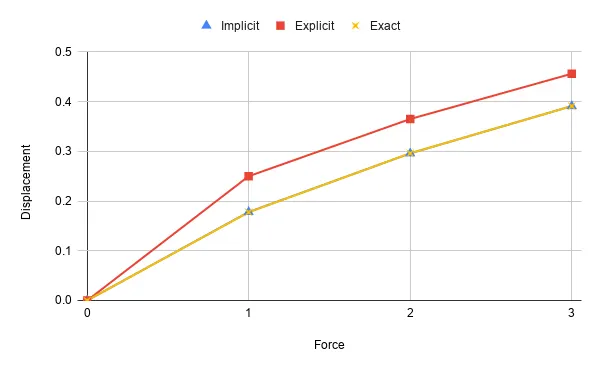
From the plot, we can observe that the implicit method gives a solution very close to the exact solution while the explicit method drifts away from the exact solution. The drift from the exact solution illustrates the lack of equilibrium between the internal and external forces. However, with smaller time steps, the explicit method would close the gap between its solution and the exact solution.
Conclusion:
A simple problem is solved using the incremental explicit and implicit procedure and the results are plotted for comparison. It is evident from the results that the explicit analysis drifts from the true solution. To overcome this problem an implicit analysis is used, which includes Newton-Raphson iterations to enforce equilibrium between internal and external forces.
However, the explicit method is much simple and fast than the implicit method. And, it becomes very important for large non-linear problems such as crash analysis. In such problems, the explicit method is preferred.