Simulation of Laminar Flow through wedge-shaped pipe using OpenFOAM

SIMULATION OF LAMINAR FLOW IN A WEDGE-SHAPED PIPE USING OpenFOAM

1. AIM

Our aim is to simulate a laminar flow in a wedge-shaped pipe by writing a Matlab code that can generate a BlockMesh Dict file for computational mesh for any wedge angle and validate the Hagen-Poiseuille equation using OpenFOAM.

2. THEORY/EQUATIONS/FORMULAE USED

OpenFOAM is an open source CFD package. It is a Finite Volume Method (FVM) based tool as it can handle unstructured mesh as well.

It contains basic predefined solvers which can be used to solve our problem, but we need to make sure that correct solver is chosen.

Structure of OpenFOAM simulations

The important directories for a simulation are as follows,

1. System – It consists of various files such as Control Dict, BlockMesh Dict, fv schemes, fv solutions. It defines the mesh and discretization schemes for the simulation.
2. Constant – It consists of various files such as transport properties, boundaries. Polymesh directory is formed after running the blockMesh Dict file.
3. Time directory – It consists folder named 0 before running the simulation. The 0 folder contains files which defines the initial conditions. After running the simulation, the results at every time intervals are also saved here.

OpenFOAM solver – icoFoam is used for problem involving laminar, transient, incompressible and Newtonian fluid. So it’s suitable for flow in a wedge-shaped pipe problem.

Hagen-Poiseuille Equation

Hagen-Poiseuille equation is a fluidic law to find the head loss (or) pressure drop through a circular pipe under laminar flow conditions.

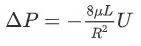
Where ΔP is Pressure drop, L is Length of the pipe, R is Radius of the pipe, U is Average Velocity of the flow and µ is Dynamic Viscosity of the fluid.

Fluid chosen for the problem – Water

Reynolds Number –It is a ratio of inertial forces to the viscous forces. It is a dimensionless number used to categorize any fluid where viscosity plays an important role, as viscosity controls the velocity.

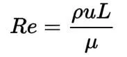
Where Re is Reynolds number, ρ is Density of the fluid, L is Length of the pipe, u is flow speed and µ is Dynamic Viscosity of the fluid.

The dimensionless number is used to determine if a fluid is laminar or turbulent. It is assumed that,

Re ≤ to 2100 is laminar flow.

Re ≥ to 2100 and ≤ to 4000 is Critical flow.

Re ≥ to 4000 is Turbulent flow.

Hydrodynamic Length

For an Internal flow in a cylindrical pipe, flow region can be divided into two phases, initial phase - Hydrodynamic entrance length and then fully developed region as shown in the below figure.

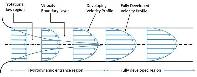
The velocity profile in laminar flow inside a pipe is parabolic in nature. But, initially the velocity profile looks like a straight line as velocity at center and at boundary are equal and parabolic nature can be seen in fully developed region.

So the length of the pipe for the problem is decided based on the Hydrodynamic entrance length, Le.

Analytical Calculation

Diameter = 0.01 m (Assumed)

Total Length of the pipe, L = Le + X = 2 m, where Hydrodynamic entrance length, Le = 1.05 (As per above equation) and for fully developed region X = 0.95 (Assumed)

Dynamic Viscosity of Water = 9.5320e-4 kg/ms

Density of Water = 997 kg/m3

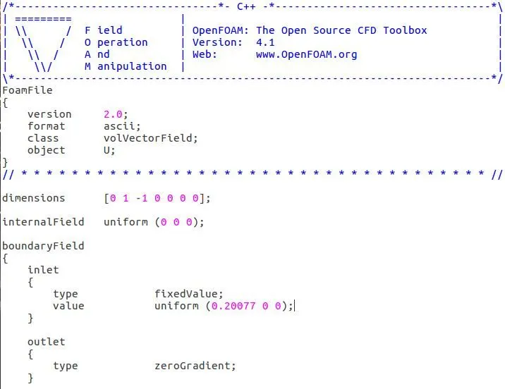
Average Velocity of the flow = 0.20077 m/s

Maximum Velocity of the flow = 0.40155 m/s

Pressure Drop (As per Hagen Poiseuille eq) = 122.48 Pa

3. OBJECTIVES & PROCEDURE

1. The main objective is to simulate a laminar flow in wedge-shaped pipe by using OpenFOAM solver and understand the flow behavior at the boundary layer and validate the Hagen-Poiseuille equation by plotting velocity profile at different locations of the wedge-shaped pipe.
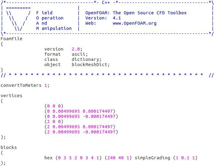
2. In the process, firstly the geometry is created by defining the vertices of a coordinate system in the blockMesh Dict file.
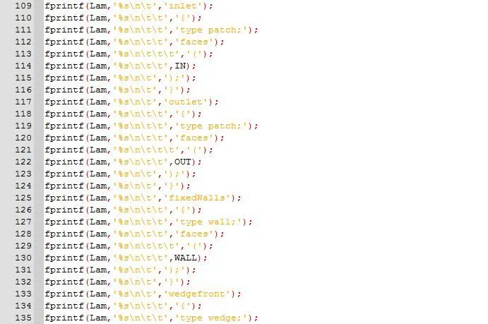
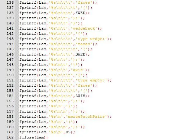
3. BlockMesh Dict file is created by writing Matlab code, which can generate BlockMesh Dict file for computational mesh for any wedge angle and mesh grading. Three different cases are defined with wedge-angle 4 deg, 3 deg and 2 deg.
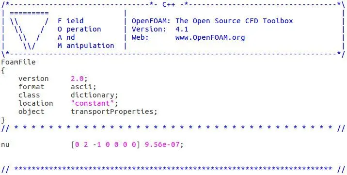
4. After getting the BlockMesh Dict file the Polymesh folder is generated and transport property i.e., kinematic viscosity is defined in the constant directory.
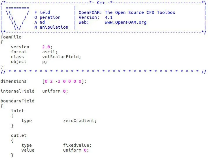
5. Then the initial and boundary condition are defined as per the problem. The primitive variables such as Velocity and Pressure are calculated using the solver.
6. Velocity contours and plot are generated and analyzed.

4. NUMERICAL ANALYSIS (Software used – OpenFOAM 4.1)

Geometric Modeling

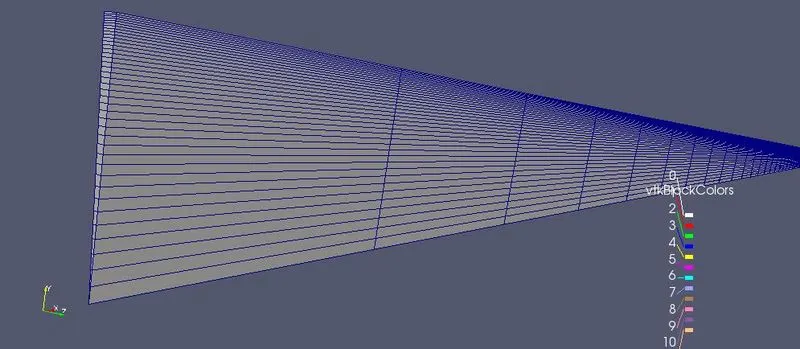
The 3D geometry is considered as one complete block and grids are defined only on two axes as the flow with respect to wedge angle is ignored.

3D Geometry – Wedge-shaped Pipe less than 5 deg

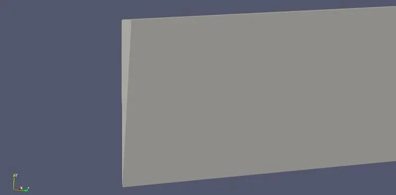
Number of Cells Mesh specification

1. X axis – 240 Grading Factor on the Y-axis – 0.1
2. Y axis – 40
3. Z axis – 1

Matlab Code for generating BlockMesh Dict file

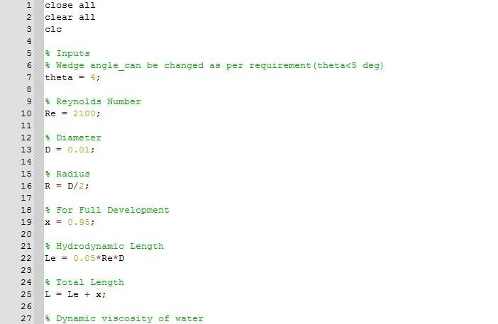
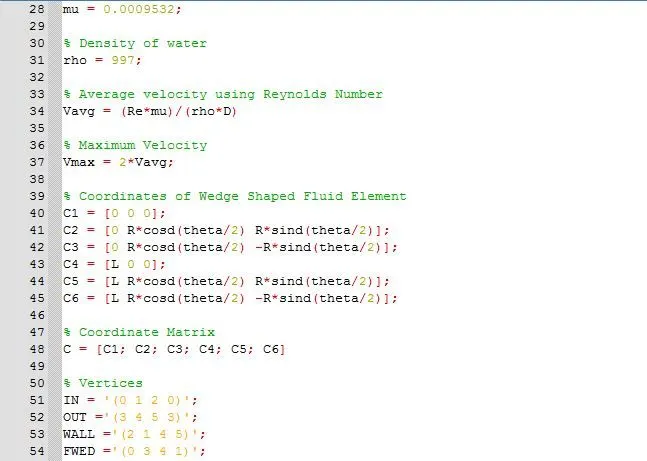
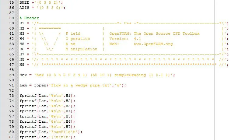
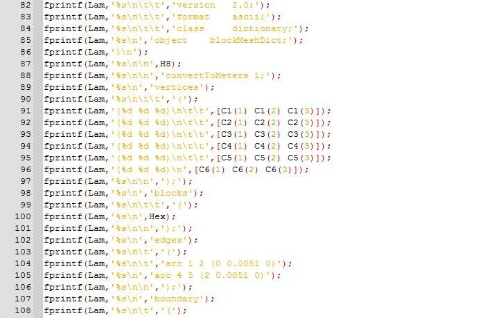
BLOCKMESH DICT FILE GENERATED FROM MATLAB

MESHING

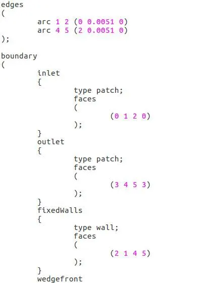
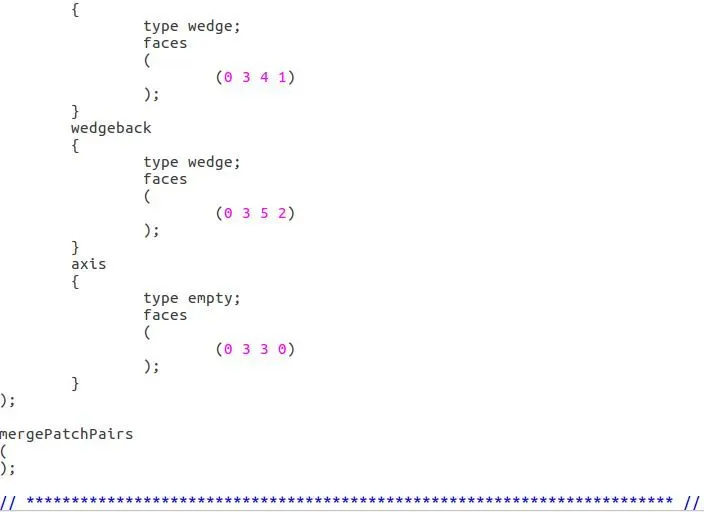
Boundaries

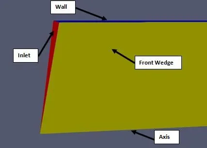
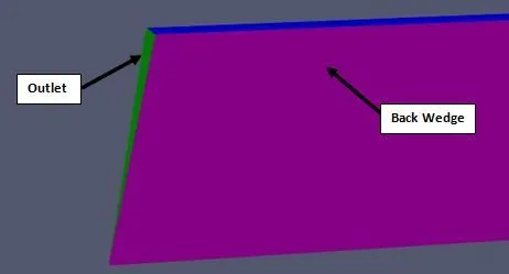
Boundary Condition

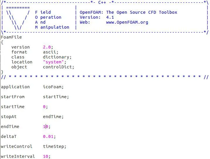
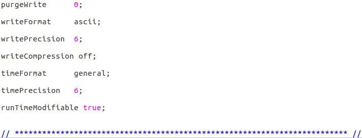
Control Dict

Transport Properties

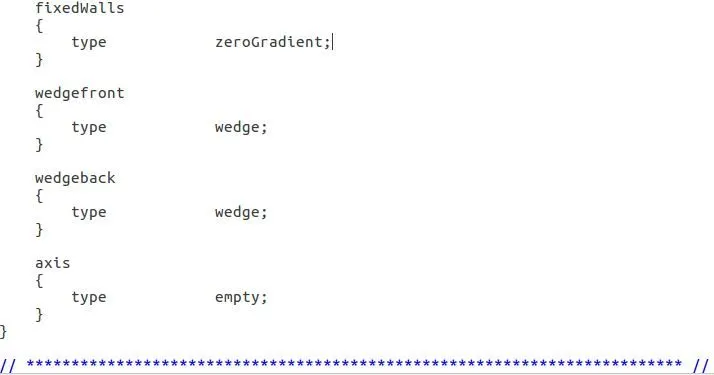
Initial Condition - Pressure

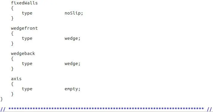
Initial Condition – Velocity

5. RESULTS

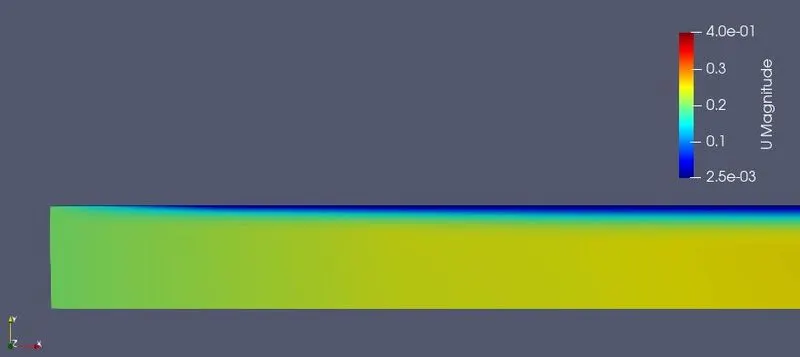
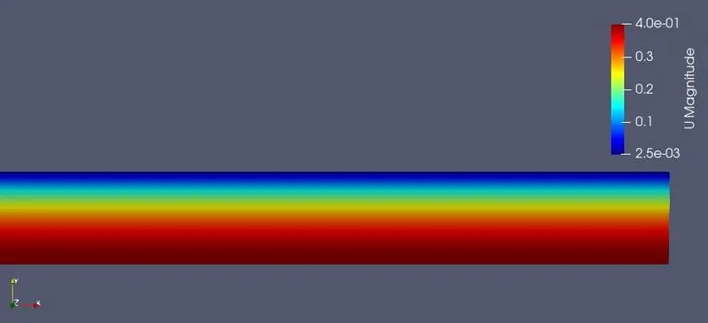
Velocity Contour of 2 Deg Wedge

Inlet

Outlet

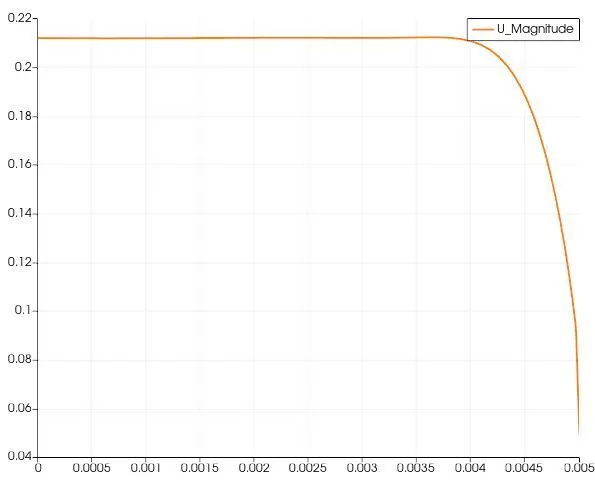
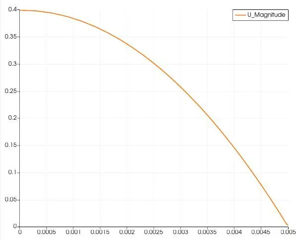
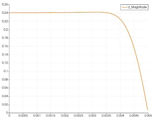
1. Velocity Plot at 0.005m
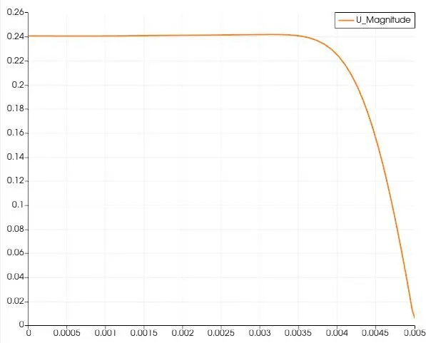
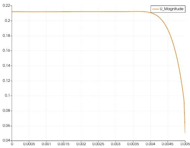
2. Velocity Plot at 0.02m
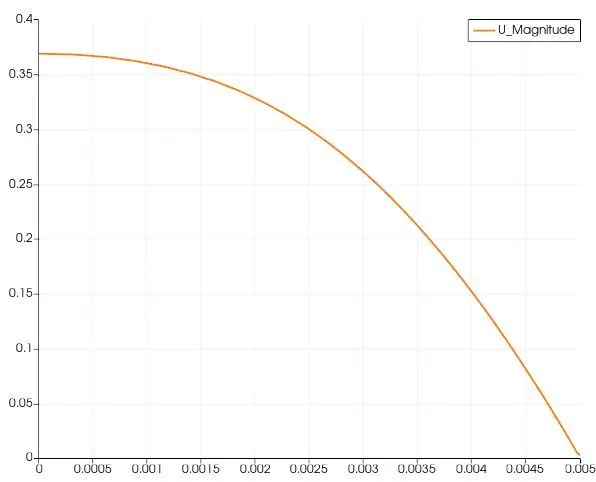
3. Velocity Plot at 0.5m
4. Velocity Plot at 1.5m

Velocity Contour of 3 Deg Wedge

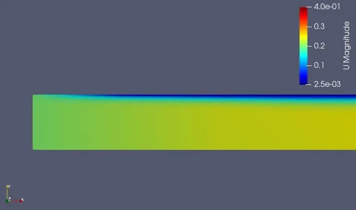
Inlet

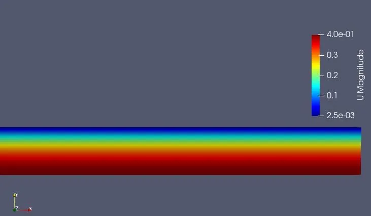
Outlet

1. Velocity Plot at 0.005m
2. Velocity Plot at 0.02m
3. Velocity Plot at 0.5m
4. Velocity Plot at 1.5m

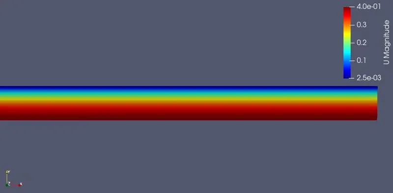
Velocity Contour of 4 Deg Wedge

Inlet

Outlet

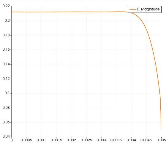
1. Velocity Plot at 0.005m
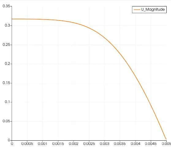
2. Velocity Plot at 0.02m
3. Velocity Plot at 0.5m
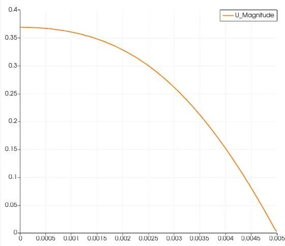
4. Velocity Plot at 1.5m

Shear Stress Plot

Velocity profile for the complete pipe

6. CONCLUSION

1. The flow in a wedge-shaped pipe problem is solved for velocity with different wedge angles using icoFoam solver in OpenFOAM.
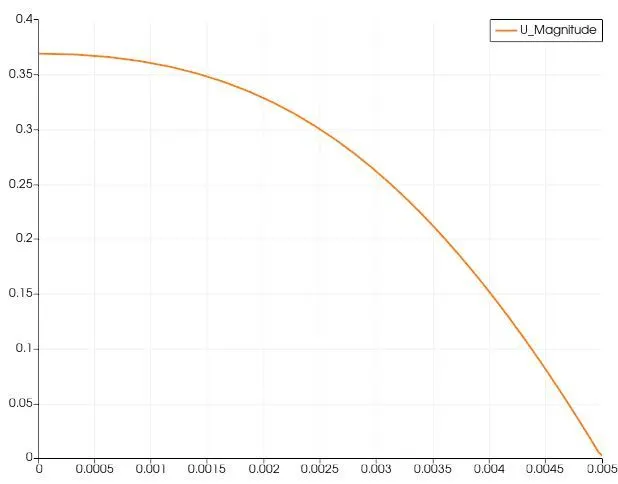
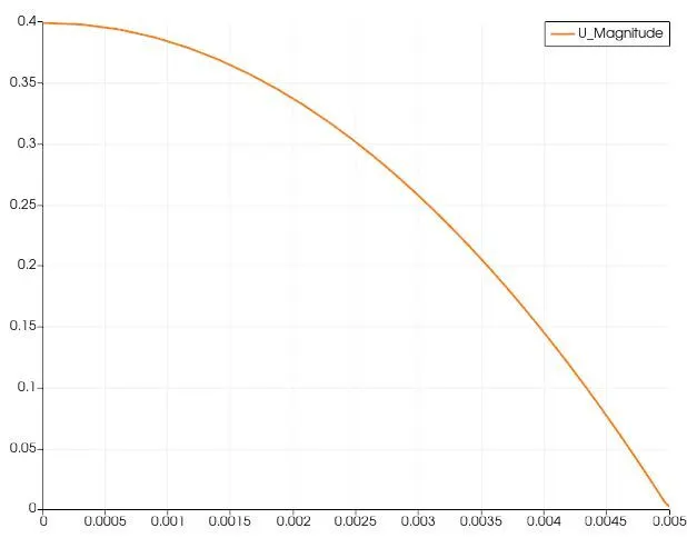
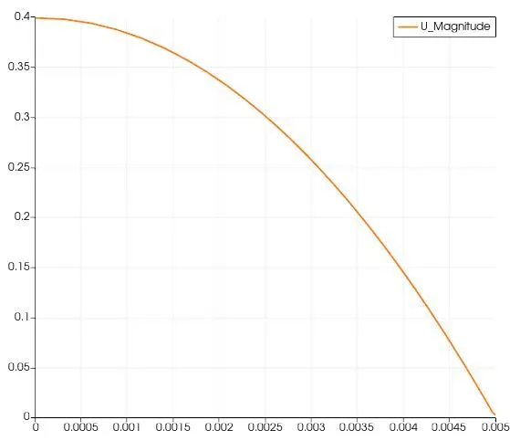
2. Graphs shows the velocity profile along the radius of wedge-shaped pipe at x=0.005 m, 0.02 m, 0.5m, 1.5m of wedge angle 2, 3, and 4 deg respectively.
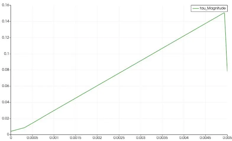
3. The shear stress on the walls is determined and plotted in post processing using paraview by calculating the velocity gradient and multiplying with the dynamic viscosity.
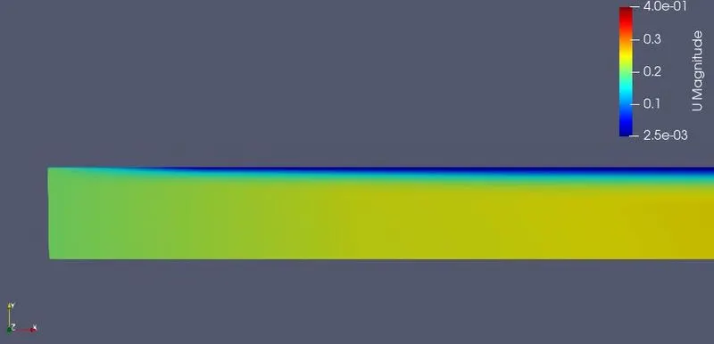
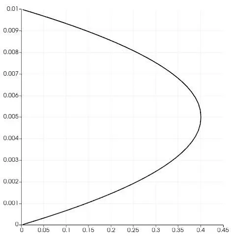
4. Graphs show that the velocity at the inlet is more of a straight line but as the flow crosses the hydrodynamic length the velocity profile becomes parabolic and this region is the fully developed region.
5. The velocity profile and hydrodynamic length are in good corelation with the analytical solution in all three cases of different wedge angles.