Week-11 Challenge: Braking
The most important feature of electric vehicles and hybrid vehicles is their ability to absorb, store and reuse the braking energy. A successfully designed braking system for a vehicle must always meet two distinct demands. While applying the sudden brake, the vehicle must come to rest in the shortest possible distance and at the same time, the vehicle must have control over the vehicle’s direction. The first one requires that the vehicle braking system be able to provide enough braking torque on all wheels. The second demand requires braking force to be distributed on all the wheels equally.
Here, the braking torque required is much larger than the torque that an electric motor can produce. So in order to bring the two demands success in EV and HEVs, both the mechanical braking system and electrical braking system should consider as major roles.
What is braking?
- Braking is a generic term used to describe a set of operating conditions for an electric drive system. It includes rapid stopping of the electric motor, holding the stopping of the electric motor, holding the motor shaft to a specific position, maintaining the speed to the desired value, or preventing the motor from overspeeding.
A regenerative braking system is the electrical braking of a vehicle using motors as brakes. The total kinetic energy which is to be utilized by the wheels travel a certain distance was being stopped by for some reason by the braking system then the accumulated energy near the power train is directed to travel back to the energy storage through the motor. So here the motor acts like a generator that stores mechanical energy into electrical energy in the battery. This stored energy can be reused by the electric motor for vehicle propulsion. This regenerative system improves motor efficiency by simply converting kinetic energy into electrical energy which is to be generated as heat energy during frictional braking.
If a 1500kg vehicle traveling at 70km/h has 300kJ of kinetic energy, which drops to zero as the vehicle comes to rest. If we can utilize this recovered it would be enough to propel the same vehicle for 1.8km at 70km/h.
This will significantly recover energy which leads to increased vehicle range.
Driving cycle:
The range of the electric vehicle is a major problem in the design of any electric vehicle.
Two types of tests can be performed with regard to the range of a vehicle.
- Constant velocity test
- The vehicle is driven in reality or on simulation, through a profile of ever-changing speeds.
These driving cycles have been developed in order to provide a realistic and practical test for the emissions of vehicles. One such is the LA-4 cycle which is based on actual traffic lows in Los Angeles CA which last for 1500 seconds, and for each second there is a different speed. SFUDs are of a similar type for a short duration of 360second but have the same average speed, the same proportion of time stationery, the same maximum acceleration, and braking, and give very similar results when used for simulating vehicle range.
The ECE-15 dive cycle which is a European cycle tends to be rather simpler, with periods of constant acceleration and constant velocity, is useful for testing the performance of small vehicles such as battery-electric cars. The EC emission tests have to be combined with the extra-urban driving cycles (EUDC) of a maximum speed of 120km/h.
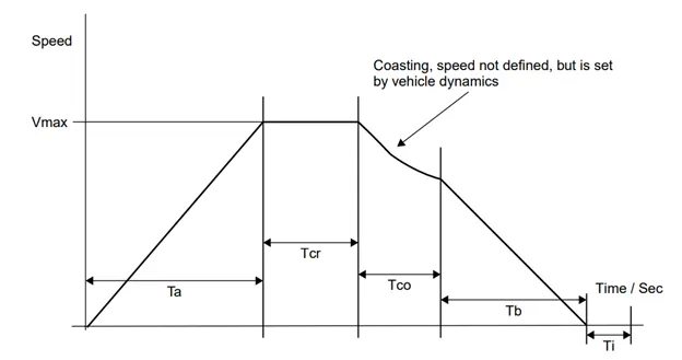
SAE J227a is a standard driving cycle, which has four versions, with different speeds. Each cycle is quite short in time and consists of an acceleration phase, a constant velocity phase, a coast phase, and a braking phase, followed by a stationary time. In the coasting phase, where the speed is not specified, n=but tractive effort is set to zero.
Braking Energy calculation:
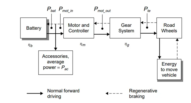
The ratio of E2/E1 gives the percentage of energy that is returned to the vehicle by using regenerative braking. E1 is the total energy lost (kinetic and potential energy) during the braking process, while E2 is the energy recovered and returned to the battery.
Braking energy can be calculated by integrating the braking power
Eb=integral Pb dt
The equation for braking power,

Where m is the mass in kg
V is the speed in m/s
Fr is rolling resistance
Rho ais air density
Theta is the grade angle
Cd is aerodynamic drag
Ar is the frontal area
Braking power is extremely important in regenerative braking controller design, as regenerative braking should only be applied within a certain power limit as well as depending on the battery state of charge. High power values present a danger to the battery because recharging too fast lowers a battery’s life.
Let us consider the ECE-15 fuel economy testing cycle:
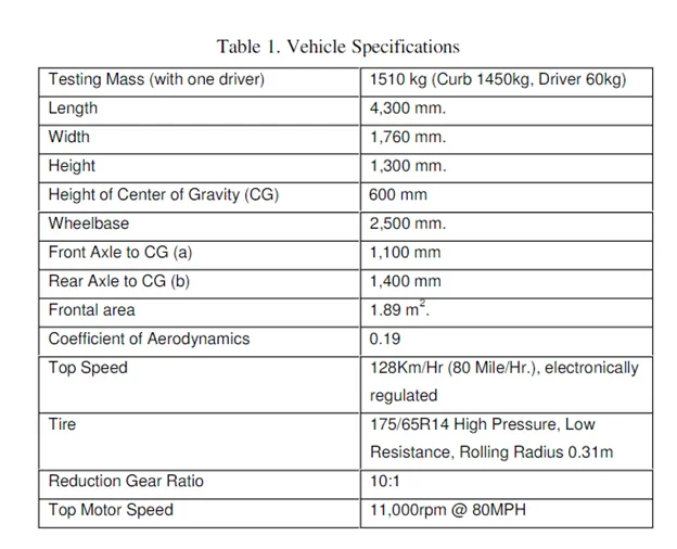
ECE-15(ECE R84) fuel economy testing cycle has 15 working conditions as shown the below figure. Four of the fifteen working conditions in the cycle are decelerations that are highlighted
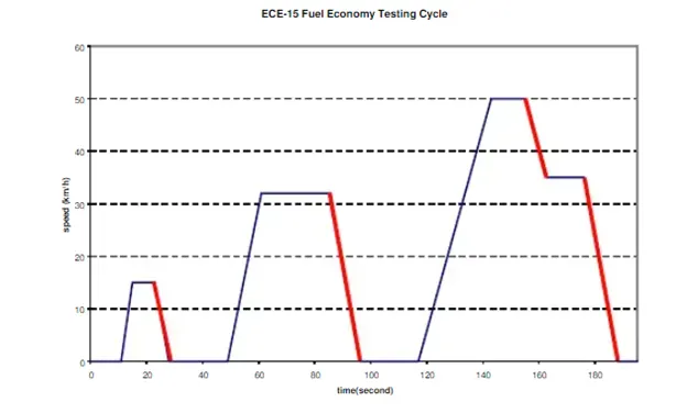
The specifications for the four decelerating conditions are
Vehicle speed Time
1 15 km/h-0km/h(9.37mph-0mph) 5 seconds
2 32 km/h-0km/h(20mph-0mph) 11 seconds
3 55km/h-35km/h(34.375mph-21.875mph) 8 seconds
4 35 km/h-0km/h(21.875mph-0mph) 12 seconds
The performance of regenerative braking in each deceleration condition and its overall performance are listed
In the high band, the torque is limited by the limit of the power output of the motor/inverter system. It initially decreases rapidly, but the decreasing rate slows down. The eV has a maximum speed of 80m/h corresponding to the red line speed of 11,000 rpm of motor, which is also a cutoff lie of regen torque. The polynomial approximation in this brand is.

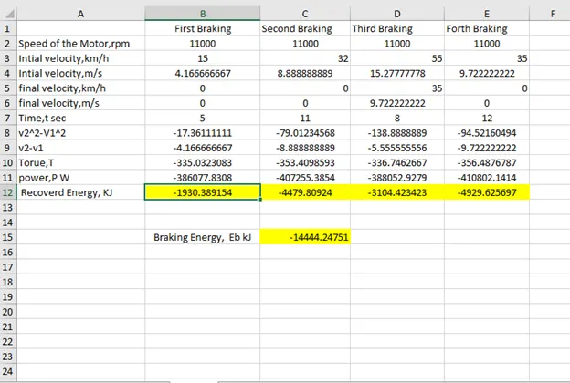
For the first braking period,
`Tv2-v1=frac{dT}{dV}=-0.0357*V^2+8.71456*V-317.49` V2=0 and V1=15km/h
=-333.5 N-m/s
Power, P=`frac{2*phi*N*T}{60}` where N-11,000rpm
=-386077.831KW
Braking energy, E=`frac{P*t}{1000`KJ where t is the time taken.
=-1930.39 KJ
Similarly, calculate the energy for other braking periods using an Excel calculator. The total braking energy is calculated by adding all recovery energy during four braking periods.
Q2. Why electric motor can’t develop braking torque at a high speed similar to starting? How electric and mechanical brakes are coordinated?
A.
As the motor will have rated speed when the vehicle speed increases beyond the rated speed the torque decreases and cannot attain the required brake torque demand as it was given at starting speed.
So, the electric motor cannot develop braking torque at high speed because wheel lock-up can happen which is not recommended as it is harmful to the vehicle. In such a situation, mechanical braking can be assisted to reach the required brake torque demand. So, there will need of both electrical braking and mechanical braking at high speed.
Electric and Mechanical braking :
In hybrid electric vehicles, there exists designed braking controllers that combine electrical braking with mechanical braking which is nothing but hydraulic, friction braking in order to provide comfortable drive, recover maximum energy and safety. This is because regenerative braking is not adequate in all situations, especially when rapid deceleration is necessary. The purpose of this combination is first to achieve desired deceleration without locking either wheel mainly the rear wheels. The second is to maximize energy recovery.
When a heavily loaded vehicle (1500kg) needs an emergency braking from speed 70km/h at 0.8g, the braking power may reach 250KW which is highly harmful to the battery and this excess amount of energy needs to be directed to some other means like a flywheel storage device (also for regeneration) otherwise it would affect the system.
But in EV’s excess energy is dissipated by friction brakes. Very high energy recovery rate is theoretically possible by regenerative braking so hydraulic braking is used for rapid deceleration even though regenerative braking is responsible for most of the deceleration of the vehicle.
We can only recover energy from the front wheels and 35% of energy dissipated due to friction braking at rear wheels is still not available for regeneration. This is because vehicles are front-wheel drives so the motor receives regenerative braking torque from the front axle. For this reason, the system is constructed based on a dual-circuit hydraulic system that groups 4-wheel disc brakes in LF-RR and RF-LR lines. The Braking Torque Control Module (BTCM) manages the braking torque between the two torque sources which also implements ABS when the wheels are locked up.
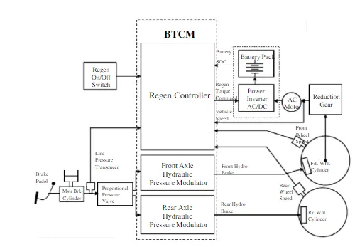
Brake System Layout
Depending on the available input, BTCM manages brake torque distribution and blending and calculates the demanded vehicle deceleration and total braking torque, and divides them into the regen demand and hydraulic torque. The hydraulic torque again split for the front and rear axles.
Regenerative braking has been integrated with anti-lock mechanical braking which contains an Anti-skid control system that deactivates the regenerative braking momentarily when the slip is detected to provide better deceleration.
In a regenerative braking system, most of the wheel lock-up happens with high brake torque demand, which requires the assistance of friction braking. In the case of very low road traction, such as road coefficient of friction as low as 0.1 only motor braking torque will be high enough to lock upfront wheels. The rear wheels will not provide any braking force so that the vehicle will lose steering and stop at an excessively large distance. Therefore, the controller has to disable regenerative braking and brake entirely by friction. This allows the sophisticated ABS brake system to maintain stability and maneuverability of the vehicle and provide maximum braking force.
Torque management of both the electrical and braking system in two scenarios:
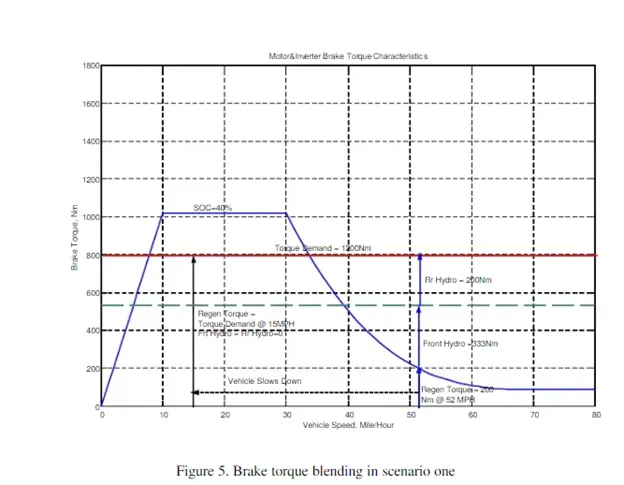
- Brake torque Demand can be lower than the regen capacity limit. Assuming a battery SOC at 40%, with the speed of 52MPH, the BTCM sensed a brake line pressure that corresponds to a constant brake torque request of 1200N-m. At this speed the regen torque upper limit is as low as only 200N-m, so most of the torque has to be generated by the hydraulic system to obtain an overall front/rear brake torque ratio of 2:1. As the vehicle slows down the Regen torque continues to increase following the polynomial curve and the hydraulic front brake torque decreases at the same rate to maintain the torque demand. At 37MPH the Regen not only has taken over the duty of front hydraulic but also partially rear during this time the hydraulic brakes of both front and rear are deactivated. This will continue until the Regen torque decrease again in the low-speed band and the capacity limit again becomes lower than the torque demand. During this time when all the brake is Regen, the vehicle recalls energy from braking at the highest efficiency because no friction braking is used.
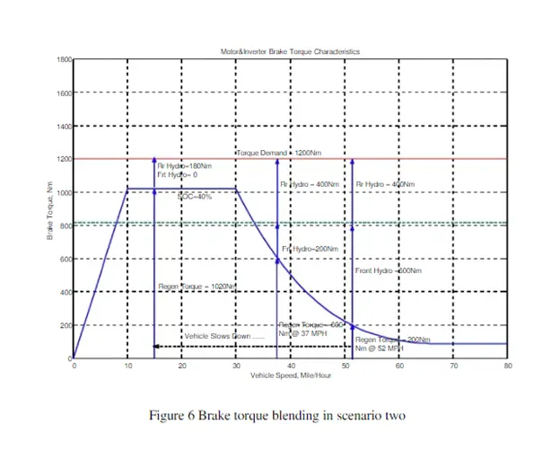
2. In the case of a high brake torque demand which is more than the regen braking limit, such as 1200N-m at 405 SOC, even though the Regen is at the highest output, the hydraulic brakes have to be applied to assist in attaining brake torque demand. So, from the initial speed of 37MPH to the end of 15MPH, the regen brake torque varies with its capacity limit and the remaining is obtained from front and rear hydraulic brakes.
3Q. Make a MATLAB program that plots the contour of given motor speed, torque, and efficiency values. Attach the codes as a .m file attach a screenshot of all plots.
A.
The major sources of loss in all types of the electric motor are divided into four main types
- Copper losses: caused by the electrical resistance of wires of the motor which dissipates heat.
Copper losses, Cu_Loss=`Kc*T^2` where Kc is constant depending on the resistance of the brushes and the coil and also magnetic flux.
- Iron Losses, Iron_Loss: These are caused by magnetic effects in the iron of the motor, particularly in the rotor.
Iron losses, Iron_Loss= `Ki*omega` where Ki is not constant as its value is affected by magnetic field strength
- Friction and windage losses Ml: these are caused by the friction torque in the bearings and brushes of the motor and the rotor will have wind resistance. The friction force will be constant but windage will be changing with the square of the speed
Windage losses =`Kw.omega^3`
- Constant losses,C: these losses occur when the motor is stationary and vary neither with speed or torque.
Total losses= `Kc*T^2+Ki*omega+Kw*omega^3+C`
Motor efficiency, Eff_motor=output power/input power
=output power/output power+ Total Losses
=`frac{Tw}{Kc*T^2+Ki*omega+Kw*omega^3+C`
Suitable values for the constants in this equation can be found by experimentation or by regression using measured values of efficiency.
`Kc`=0.8,`Ki`i=0.1, `Kw`=0.00001 C=20
It is used to plot the values of efficiency on a torque-speed graph which is sometimes known as an efficiency map for the motor which gives an idea of the efficiency at any possible operating condition
Efficiency are taken in the range of Eff_Range=[50%,60%,70%,80%,85%,90%,95%]
Using the Contour function, we can plot a three-dimension graph of efficiency in torque speed plot.
contour(S,T,Eff_motor,Eff_Range);
The two power characteristics are plotted against Torque speed characteristics and output power changing in Z direction.
P=[7000, 10000];% two values of power are taken
contour(S,T,Output_Power,P);
MATLAB code:
s=linspace(1,1000); % speed
t=linspace(1,120); % Torque
Kc=0.8; % coefficient of copper Losses
Ki=0.1; %coefficient of  Iron_Losses
Kw=0.00001;% coefficient of windage _losses
C=20;   % constant losses
[S,T]=meshgrid(s,t);
Output_Power=(S.*T);% power deliverd by motor to the shaft
Cu_Loss=(Y.^2)*Kc; % copper losses
Iron_Loss=X*Ki;  % iron losses
Wind_Loss=(X.^3)*Kw; % windage losses
Input_Power=Output_Power+Cu_Loss+Iron_Loss+Wind_Loss+C;
Eff_motor=Output_Power./Input_Power; % Efficiency of motor

Eff_Range=[0.50,0.60,0.70,0.80,0.85,0.90,0.95]; %range of efficiencies
contour(S,T,Eff_motor,Eff_Range);
xlabel('speed_rad per sec');
ylabel('Torque_Nm');
hold on
P=[7000, 10000];% two values of power are taken
contour(S,T,Output_Power,P);

legend('show')
colorbar
Contour plot of motor speed,Torque, Efficiency:
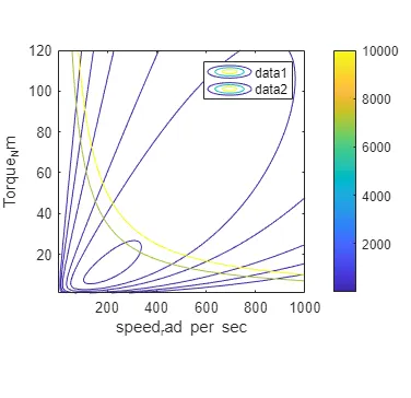
we can see two yellow curves are plotted across the graph are power curves of 7KW and 10KW and the contour plots of efficiencies are plotted against the torque-speed graph. Maximum efficiency exists at the center closed oval-shaped curve