Flow through Mixing Tee configurations to see the Mixing Effectiveness

STEADY STATE SIMULATION OF FLOW IN A MIXING TEE OF TWO CONFIGURATIONS TO COMPARE THE MIXING EFFECTIVENESS USING ANSYS FLUENT

1. AIM

Our aim is to simulate a steady state flow in a mixing tee of two configurations to compare the mixing effectiveness by selecting the suitable turbulence model and validate the numerical result with the analytical equation using ANSYS FLUENT.

2. THEORY/EQUATIONS/FORMULAE USED

ANSYS FLUENT academic version CFD package is used to carry out the simulation. It is a user friendly interface which provides high productivity and easy-to-use workflows. Workbench contains all workflow needed for solving a problem such as pre-processing, solving and post-processing.

Structure of ANSYS FLUENT simulations

The basic steps for a simulation are as follows,

1. Pre-processing – It includes geometry creation, discretization, providing named selection for using as boundary conditions. The packages used in pre-processing step are SpaceClaim, Ansys Mesher.
2. Solving – It includes applying initial and boundary conditions, adding material properties, applying suitable turbulence model as per the problem and running the iteration till convergence. The package used in post-processing step is Fluent.
3. Post-processing – It includes analyzing the results by plotting the results as charts, contour, and exporting the data, also validating the results both qualitatively and quantitatively. The package used in post-processing step is CFD-Post.

Final Temperature of the Mixture, T_mix

The equation is used to find the temperature of the mixture coming out from the Tee where the fluids of different temperature are mixed through a circular pipe under laminar flow conditions.

where m_hot , m_cold are mass flow rate of hot fluid inlet and cold fluid inlet respectively. T_{hot ,} T_cold are temperature of hot fluid inlet and cold fluid inlet respectively.

Fluid chosen for the problem – Air

Momentum Ratio – It is a ratio of velocity of the cold fluid inlet to the velocity of the hot fluid inlet.

Problem - Mixing Tee

• The simulation challenge includes two mixing tee configurations i.e., Short Tee and Long Tee.
• Each case has two momentum ratios each i.e., 2 and 4
• Hot Inlet Temperature - 36°C & Cold Inlet Temperature - 19°C

CASE – 1 SHORT TEE: Short Tee with a hot inlet velocity of 3 m/s and Momentum Ratio - 2 and 4

CASE – 2 LONG TEE: Long Tee with a hot inlet velocity of 3 m/s and Momentum Ratio - 2 and 4

Analytical Calculation

• A) Momentum Ratio – 2

Density of Air = 1.225 kg/m3

Area of Cold Inlet = 0.0002 m², Area of Hot Inlet = 0.0009 m²

Velocity of Hot Inlet = 3 m/s, Velocity of Cold Inlet = 6 m/s

Mass flow rate = Density * Cross-section Area * Velocity

Mass Flow rate of Hot Inlet, m_hot = 0.00331

Mass Flow rate of Cold Inlet, m_cold = 0.00147

Final temperature of the mixture, T_mix = 30.77°C

• B) Momentum Ratio – 4

Density of Air = 1.225 kg/m3

Area of Cold Inlet = 0.0002 m², Area of Hot Inlet = 0.0009 m²

Velocity of Hot Inlet = 3 m/s, Velocity of Cold Inlet = 1 m/s

Mass flow rate = Density * Cross-section Area * Velocity

Mass Flow rate of Hot Inlet, m_hot = 0.00331

Mass Flow rate of Cold Inlet, m_cold = 0.00294

Final temperature of the mixture, T_mix = 28°

3. OBJECTIVES & PROCEDURE

• The main objective is to simulate a steady state flow in a mixing tee of two configurations to compare the mixing effectiveness by selecting the suitable turbulence model and validate the numerical result with the analytical equation using ANSYS FLUENT.
• In the process, firstly the geometry is imported into SpaceClaim for cleanup. The fluid volume is extracted by removing unwanted faces and the suppressing them for physics to make the simulation easier.
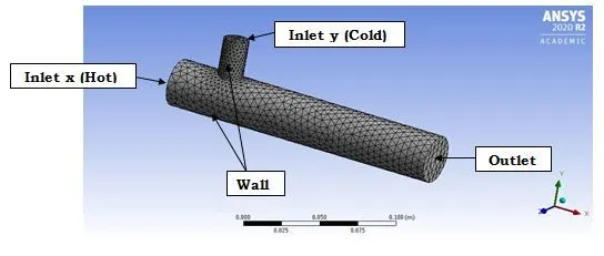
• In Meshing module the boundaries of the mixing tee are named and mesh is generated with defaults element size. Also the quality of the mesh is checked and made sure that it is good enough to carry out the current simulation.
• Then setup the solver type, the initial and boundary condition, suitable turbulence model are defined as per the problem. The primitive variables such as Velocity and Temperature are calculated using the solver.
• Temperature and Velocity contours and plot are generated and analyzed.

4. NUMERICAL ANALYSIS (Software used – ANSYS 2020 R2)

4.1 Geometric Model

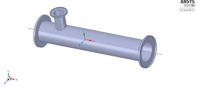
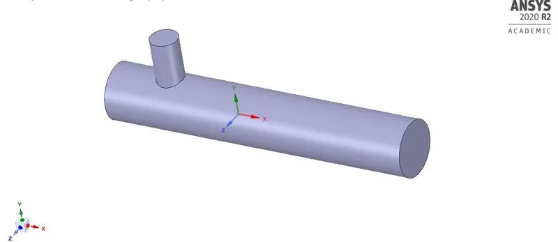
The 3D geometry part file is imported in SpaceClaim to extract the fluid volume by removing unwanted faces and the suppressing them for physics to make the simulation easier.

3D Geometry – Mixing Tee

Extracted Fluid Volume with suppression for physics

4.2 Mesh and Named selection

4.3 Solver Set-up

1. The mesh file is imported into the FLUENT software for the analysis of the modeled surface.
2. Once the mesh file is loaded and displayed, it is checked for the units, scale, and mesh.
3. There are two types of numerical solver methods pressure –based and density-based solver. The pressure based solver was used rather than the density based solver as the simulation is for lower Mach number. Absolute velocity formulation, steady state was used for the analysis.
4. Energy equation was also switched on for the analysis process as we are interested in temperature of the system.
5. K-Epsilon (2-eqn) and K-Omega (2-eqn) turbulence model was used for the first analysis to check the suitability.
6. The fluid material chosen was air.
7. Report definitions such as area weighted average, standard deviation of are set up as we are interested in the physical quantity such as temperature at the outlet, mixing effectiveness of tee.
8. Initialization is done and numbers of iterations are set for running the simulation.

Initial Setup and Boundary Condition

Zone	Type	Boundary Condition	Additional conditions (if any)
Inlet X	Velocity - Inlet	Velocity – 3 m/s, Temperature - 36°C	Steady State, Pressure Based, Absolute Switched ON Energy equation Turbulence Model – K-Epsilon (Realizable)
Inlet Y	Velocity - Inlet	Velocity – 6 or 12 m/s, Temperature - 19°C
Outlet	Pressure - Outlet	Gauge pressure of 0Pa, Temperature – 26.85°C
Walls	Wall	Stationary wall without slip

5. RESULTS

Case – 1: Short Tee Momentum ratio – 2

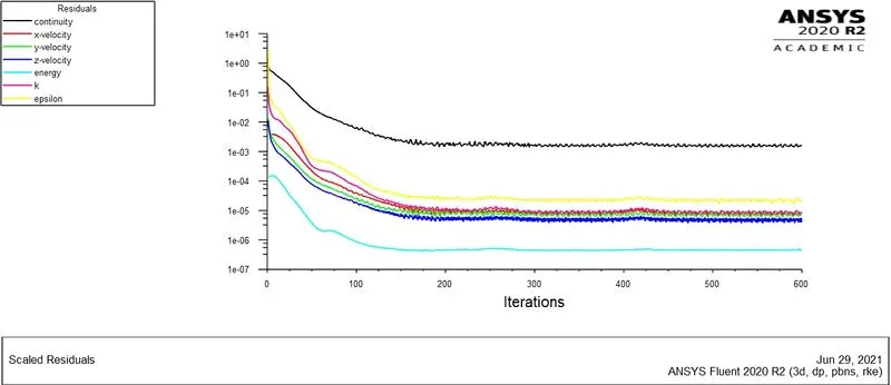
Fig: Convergence Plot

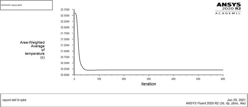
Fig: Temperature Plot

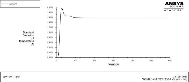
Fig: Standard Deviation Plot

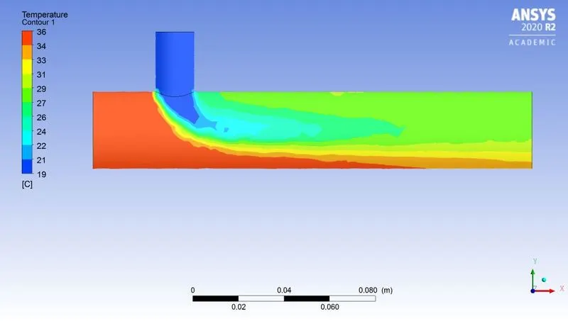
Fig: Temperature along the Tee contour

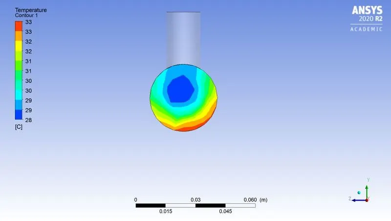
Fig: Temperature across the Tee contour

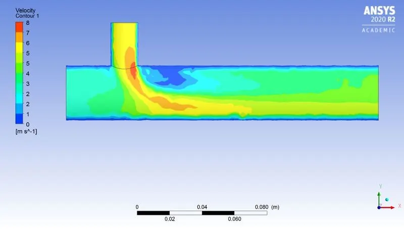
Fig: Velocity along the Tee contour

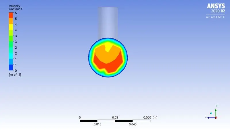
Fig: Velocity across the Tee contour

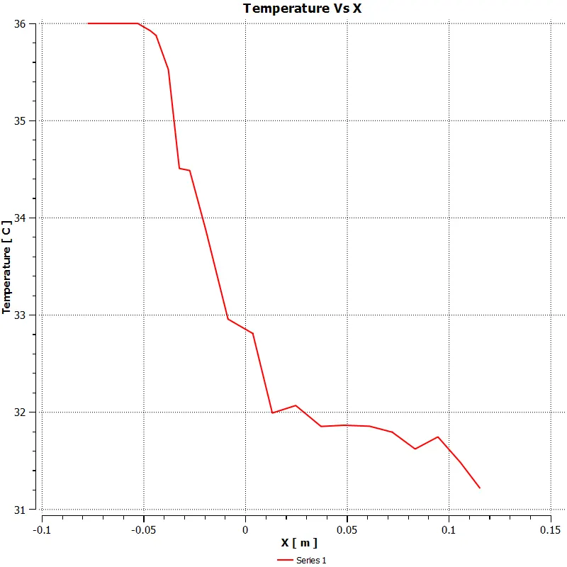
Fig: Temperature line plot using 1 seed point

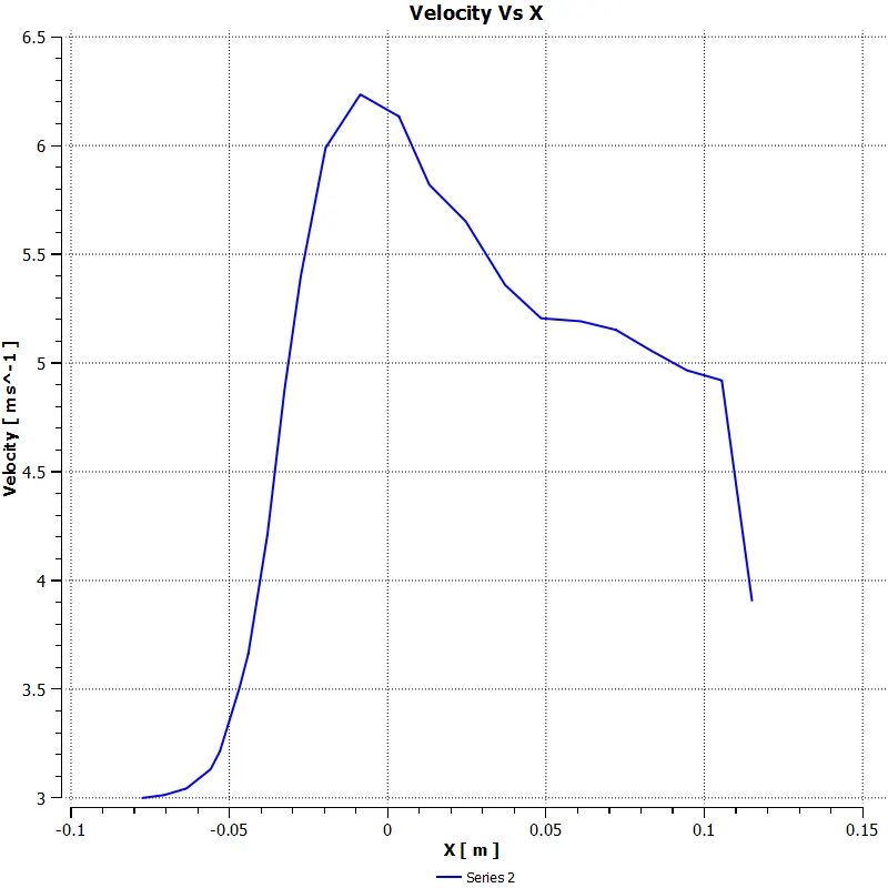
Fig: Velocity line plot using 1 seed point

Case – 1: Short Tee Momentum ratio – 4

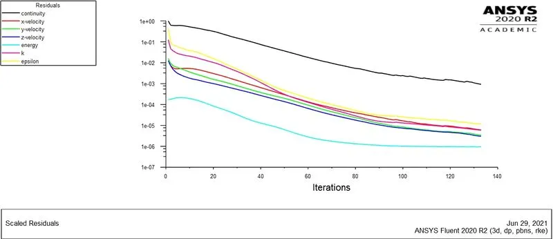
Fig: Convergence Plot

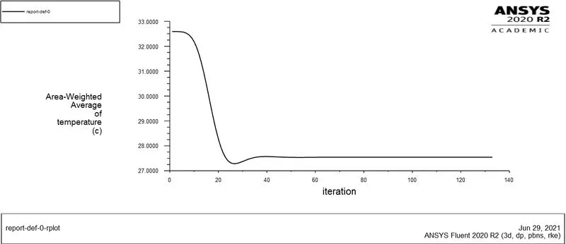
Fig: Temperature Plot

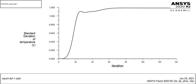
Fig: Standard Deviation Plot

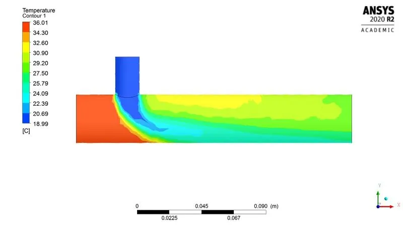
Fig: Temperature along the Tee contour

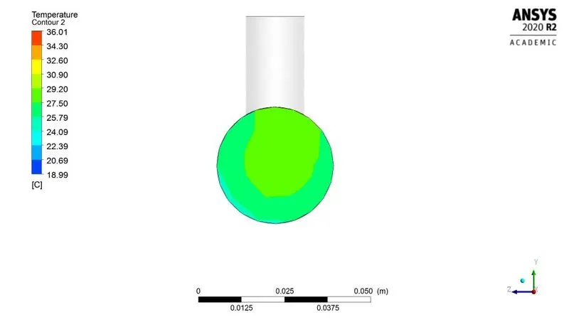
Fig: Temperature across the Tee contour

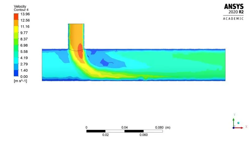
Fig: Velocity along the Tee contour

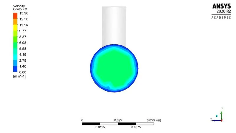
Fig: Velocity across the Tee contour

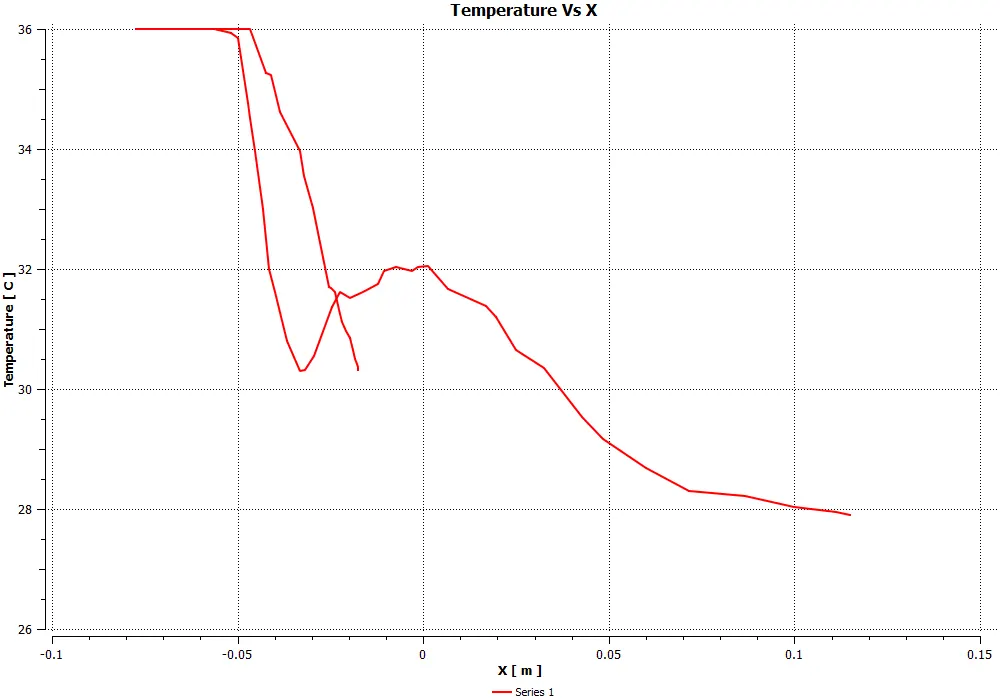
Fig: Temperature line plot using 2 seed points

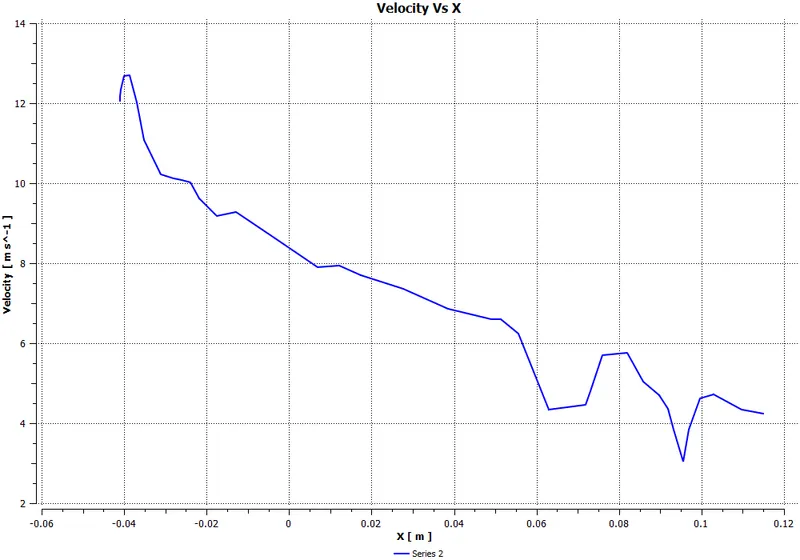
Fig: Velocity line plot using 1 seed point

Case – 2: Long Tee Momentum ratio – 2

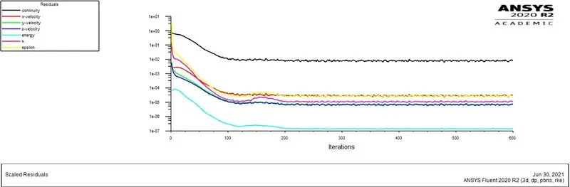
Fig: Convergence Plot

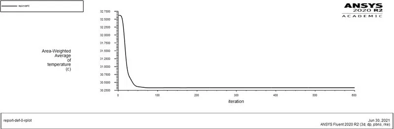
Fig: Temperature Plot

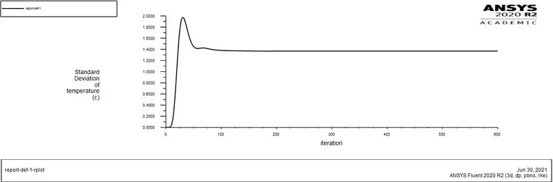
Fig: Standard Deviation Plot

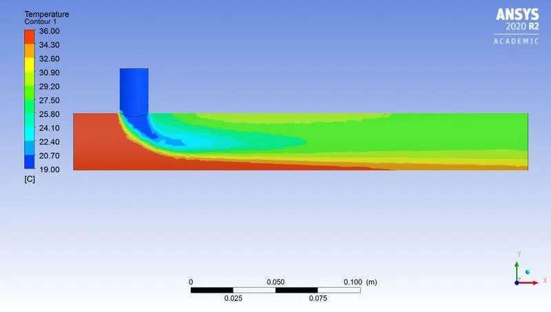
Fig: Temperature along the Tee contour

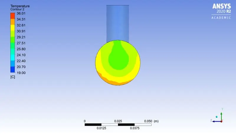
Fig: Temperature across the Tee contour

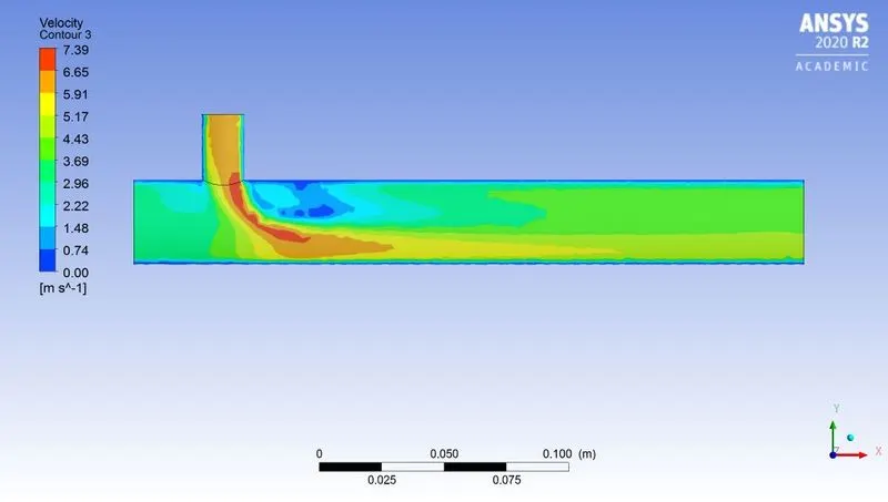
Fig: Velocity along the Tee contour

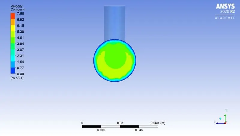
Fig: Velocity across the Tee contour

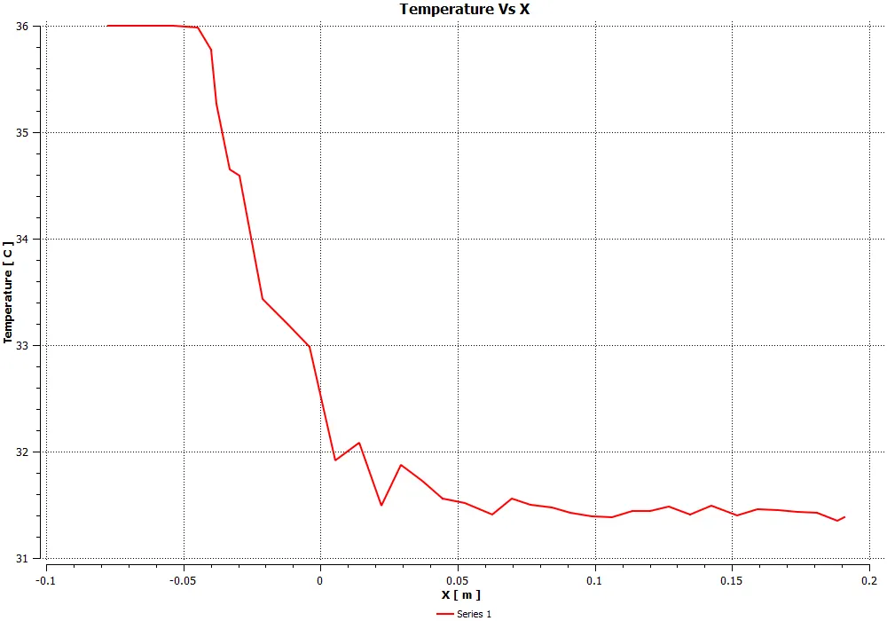
Fig: Temperature line plot using 1 seed point

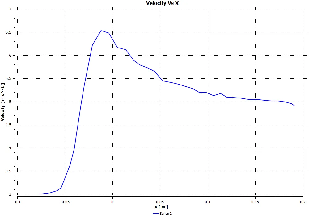
Fig: Velocity line plot using 1 seed point

Case – 2: Long Tee Momentum ratio - 4

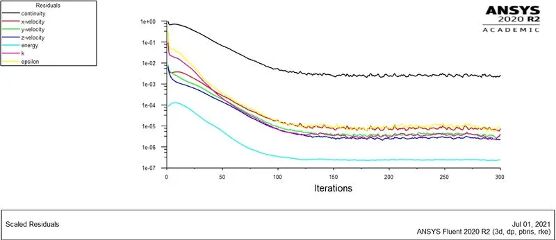
Fig: Convergence Plot

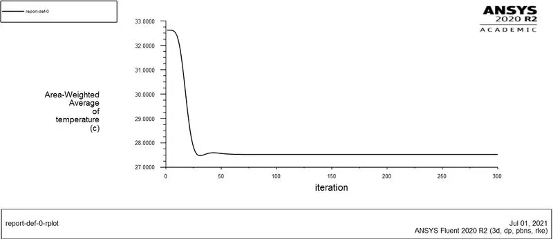
Fig: Temperature Plot

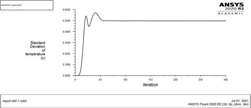
Fig: Standard Deviation Plot

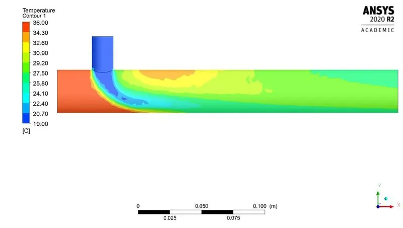
Fig: Temperature along the Tee contour

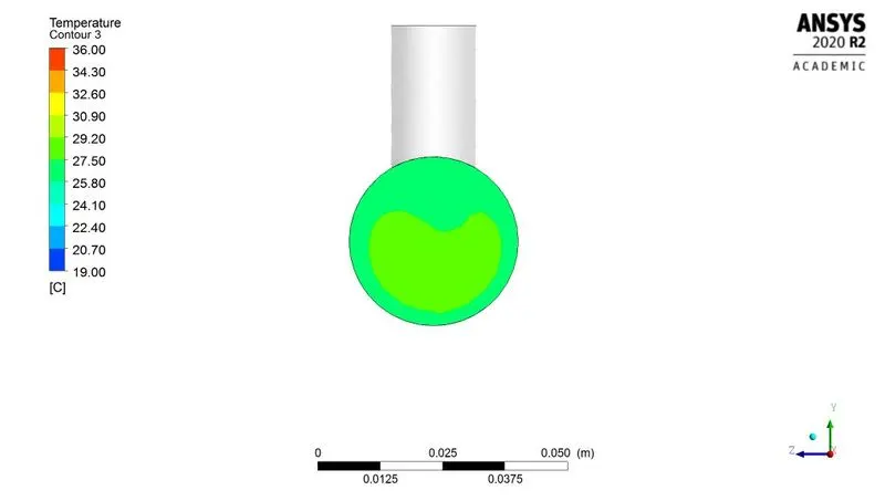
Fig: Temperature across the Tee contour

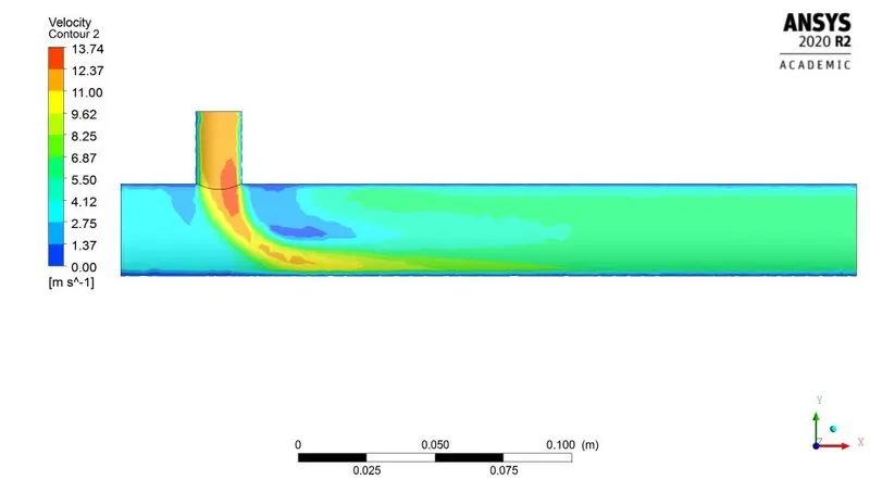
Fig: Velocity along the Tee contour

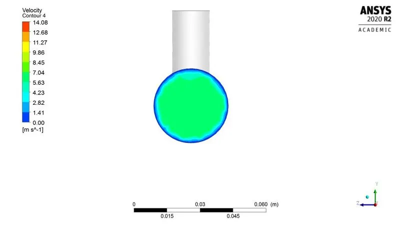
Fig: Velocity across the Tee contour

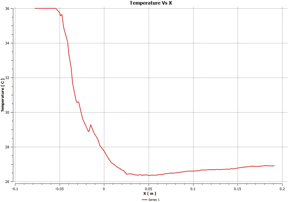
Fig: Temperature line plot using 1 seed point

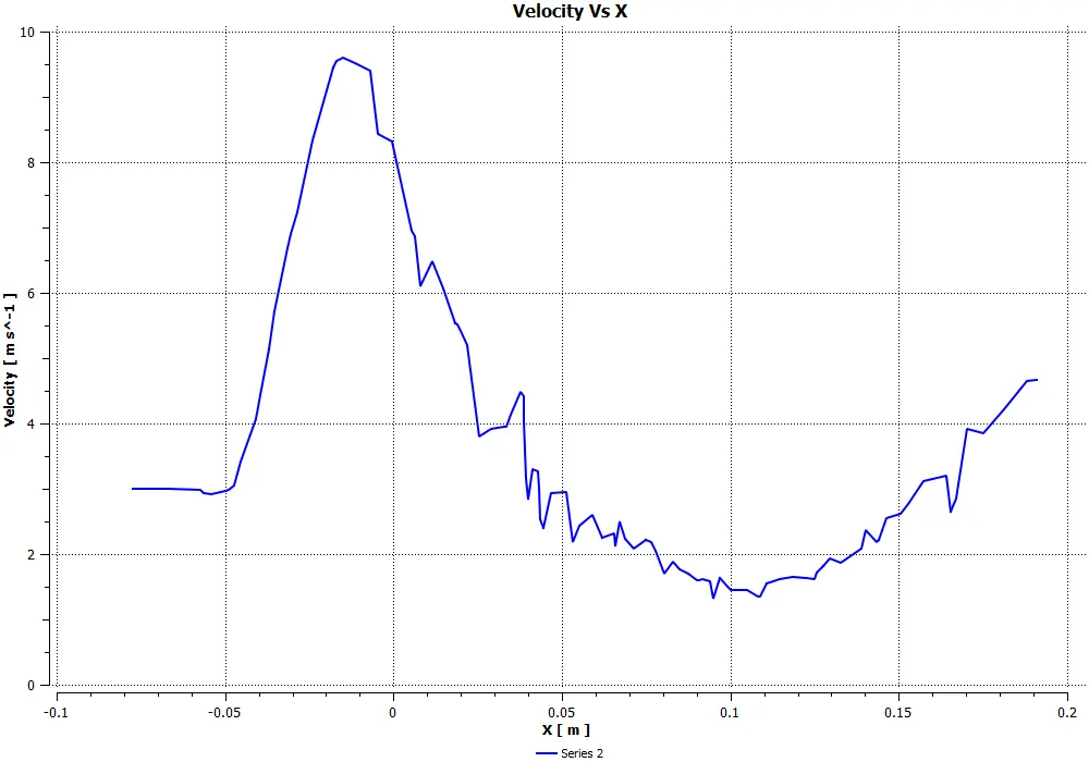
Fig: Velocity line plot using 1 seed point

Comparison of Simulation and Analytical Results

MIXING TEE SIMULATION		SHORT TEE				LONG TEE
		K-Epsilon		K-Omega SST		K-Epsilon
Sr. No.	Particulars	Momentum Ratio 2	Momentum Ratio 4	Momentum Ratio 2	Momentum Ratio 4	Momentum Ratio 2	Momentum Ratio 4
1	Cell Count	12583	12583/106253(GI)	12583	12583	56287	56287
2	Average Outlet Temp - Computational	30.25	27.5	30.25	27.5	30.35	27.5
3	Average Outlet Temp - Analytical	30.77	28	30.77	28	30.77	28
4	Number of Iterations for convergence	600	132/300(GI)	197	204	300	300
5	Standard Deviation	1.6	1.18	1.85	1.25	1.4	0.5

6. CONCLUSION

1. The steady state flow in a mixing tee problem is solved for mixing effectiveness with two different configurations and two momentum ratios in ANSYS FLUENT.
2. Initially both K-Epsilon (2-eqn) and K-Omega (2-eqn) turbulence model was used for the first case and found that outlet temperature were same but slight difference in standard deviation was observed.
3. But the main difference is that K-Epsilon is used for analysis of flow away from the walls and K-Omega is used for analysis of flow near the wall. In our case we are dealing with the flow away from the wall so K-Epsilon is the suitable turbulence model.
4. The velocity, temperature contour along mixing tee shows that small portion of high temperature fluid slips at the outlet in case of lower momentum ratio but there is no such slip in case of higher momentum ratio.
5. Also in the validation perspective higher momentum ratio results are much closer to the analytical results compared to the lower momentum ratio and more importantly the mixing effectivess is better in the case with higher momentum ratio as the standard deviation value was less.
6. Comparing the contours and standard deviation reports of both long and short tee suggests that increase in length increses the mixing effectiveness.
7. Grid independent study is done for case 1 (Short Tee with momentum ratio - 4) by increasing the number of cells (106253) by little margin and observed that simulation was not converged till 300 iterations but similar patterns were maintained for last 175 iterations.
8. Also the mixture temperature and mixing effectiveness results were similar so we can say that results are grid independent as of now. We can also check again by increasing the number of cells by higher margin given that more time and system with better performance is available.
9. So this quick simulation results shows that higher momentum ratio and increased length of mixing tee case to be an optimum model to achive better mixing effectiveness.