Week 1- Mixing Tee
Mixing Tee
Aim: To set up steady-state simulations and compare mixing efficiencies for short and long-mixing tees when the hot inlet temperature is 36°C and the Cold inlet is at 19°C.
Objective:
- Perform simulations for Short and Long mixing tees with a hot inlet velocity of 3m/s and momentum ratios of 2 and 4.
- Perform mesh independency test for any one case.
- Select an appropriate viscous model with reasoning.
- compare cell count, average outlet temperature, and number of iterations for convergence for the two cases.
- to create velocity and temperature contour and line plots along and across the pipe.
- Study the effect of length and momentum ratio on results.
Problem setup:
- case 1
- Short mixing tee with a hot inlet temperature of 3m/s.
- Momentum ratio of 2,4
-
case 2
- Long mixing tee with a hot inlet temperature of 3m/s.
- Momentum ratio of 2,4
Here the momentum ratio is defined as: $$ momentum\ ratio = \frac{Velocity\ at\ cold\ inlet}{Velocity\ at\ hot\ inlet} $$
Computation domain
Comparison of the two mixing Tee geometries:
| Geometry | Diameter inlet X | Diameter inlet Y | Length |
| Short | 33.8761 mm | 16.9626 mm | 192.3778 mm |
| Long | 33.8761 mm | 16.9626 mm | 268.328 mm |
So the difference in length between short and long tee geometry is 75.9502 mm.
Procedure:
- In the Toolbox on the left-hand side in the workbench, select and drag the Fluid flow analysis using the FLUENT solver into the Project Schematic.
- Rename the Standalone simulation tree in the schematic to whatever project we are doing at the time.
- In the geometry, open SpaceClaim and import the geometry.
- Extracting the Volume from the STEP file imported.
- Suppressing the Solid model (shell) for physics as it is not important for our simulation. (we can see the caution symbol for that part)
- Once preparing the geometry is done, load the meshing window. Suppressed part is not loaded in the meshing window.
- Create a named selection by selecting faces and naming them inlet-x, inlet-y, outlet, and walls.
- Ansys uses a bounding box and calculates the values that are filled in the mesh tab.
- use the section plan and inspect the mesh. {also use show whole elements option}
- Element quality is represented on a scale of 0-1. 0 is minimum quality and 1 is maximum quality. make sure the element quality is not less than 5%.
- pressure-based solver, velocity formulation absolute and we are going to measure temperature so turn on the energy equation.
- Select the appropriate viscous model.
- In the boundary setting edit the inlet boundary conditions as 3m/s for inlet velocity and 36°C temperature at inlet-x, as for inlet-y it is 6m/s and 19°C.
- Material is air.
- create the required plots in the solutions tab to monitor.
Mesh independency test:
First, we are going to perform a mesh independency test for one case and then use the same mesh settings for all other cases. Selecting the case 1 short mixing tee with a momentum ratio of 2.
| Element size | 10.219 mm | 5 mm | 2.5 mm | 1.5 mm |
| Cell count | 12692 | 14249 | 61233 | 213011 |
| No. of Iterations for Convergence | 89 | 113 | 102 | 86 |
| Average Outlet Temperature °C | 30.251 | 30.247 | 30.28 | 30.337 |
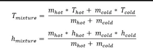
Using the analytical solution Compare the Temperature at the outlet as a parameter.
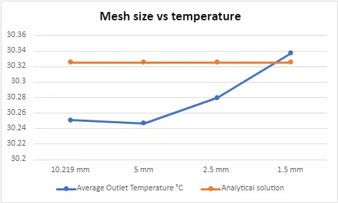
As we can see from the plot the mesh size of 1.5mm is selected for the rest of the simulations.
| K-epsilon | k-omega | |
| Element size | 1.5 mm | 1.5 mm |
| Cell count | 213011 | 213011 |
| No of Iterations for Convergence | 86 | 78 |
| Average Outlet Temperature °C | 30.337 | 30.445 |
| Analytical solution | 30.3255 | 30.3255 |
| Error | 0.04% | 0.39% |
Results:
| Case | Cell count | Convergence | Average Temperature | Average Velocity | Standard deviation Temperature | Standard deviation Velocity | Analytical |
| 1a | 213011 | 86 | 30.337 | 4.5081 | 2.5641 | 0.64687 | 30.322 |
| 1b | 213011 | 202 | 27.613 | 6.0484 | 1.4527 | 0.57547 | 27.487 |
| 2a | 289669 | 82 | 30.403 | 4.5032 | 2.0693 | 0.7243 | 30.322 |
| 2b | 289669 | 132 | 27.472 | 6.0236 | 0.70678 | 0.62787 | 27.487 |
Case 1a
| Residuals | 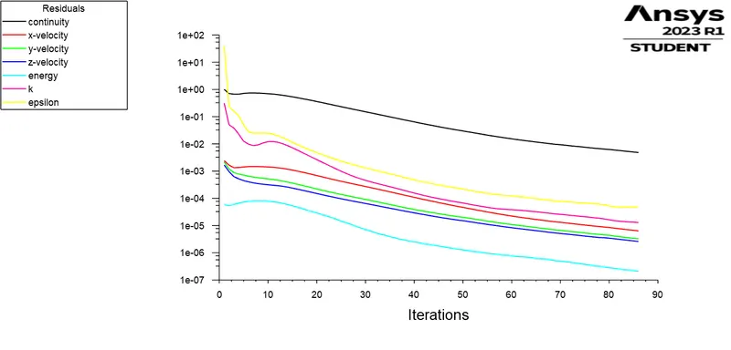 |
| Average outlet temperature | 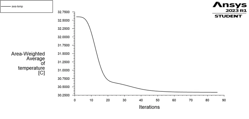 |
| Average outlet velocity | 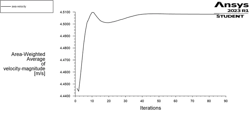 |
| Standard deviation of Temperature | 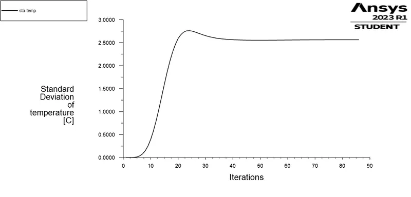 |
| Standard deviation of Velocity | 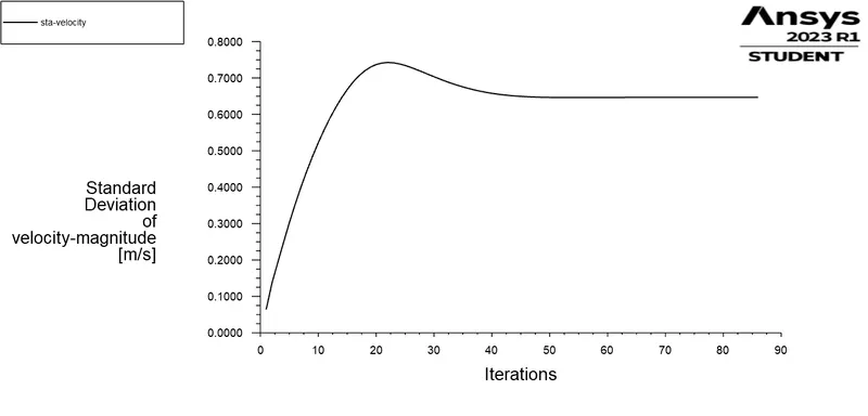 |
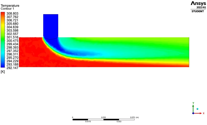
Contour plots
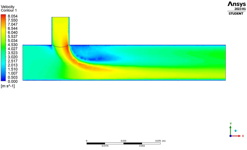
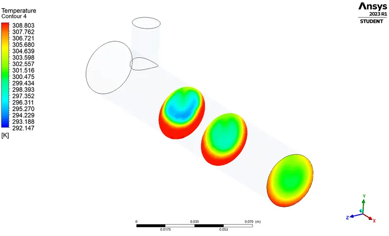
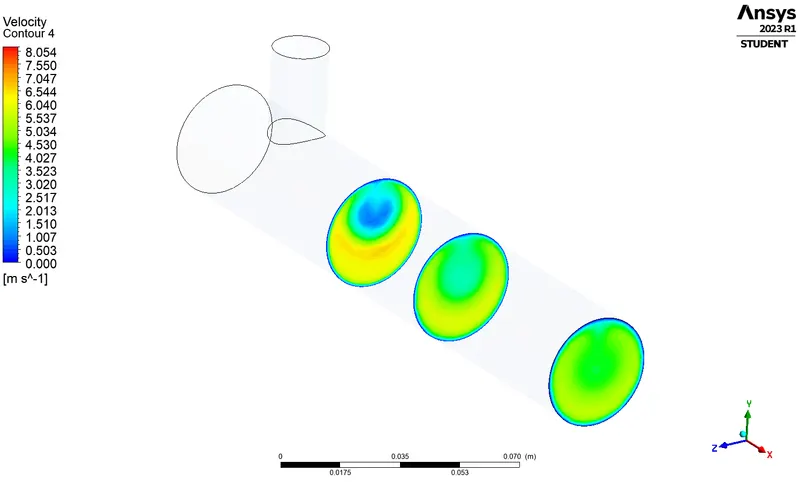
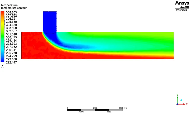
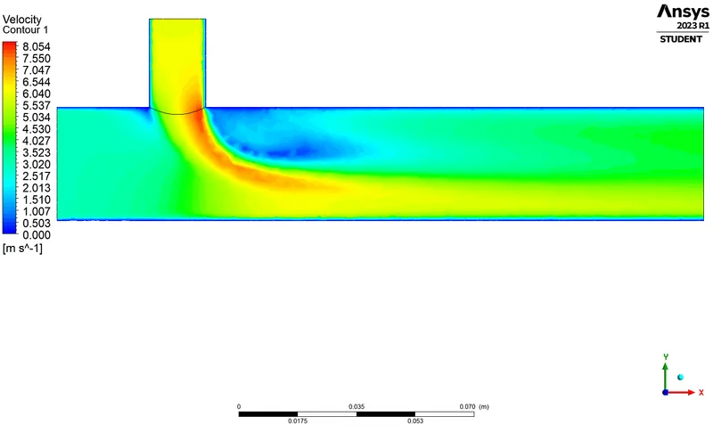
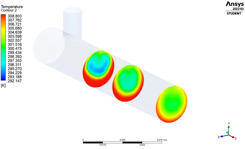
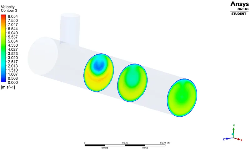
Case 1b
| Residuals | 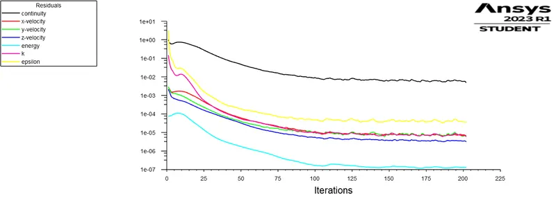 |
| Average outlet temperature | 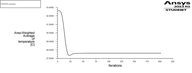 |
| Average outlet velocity | 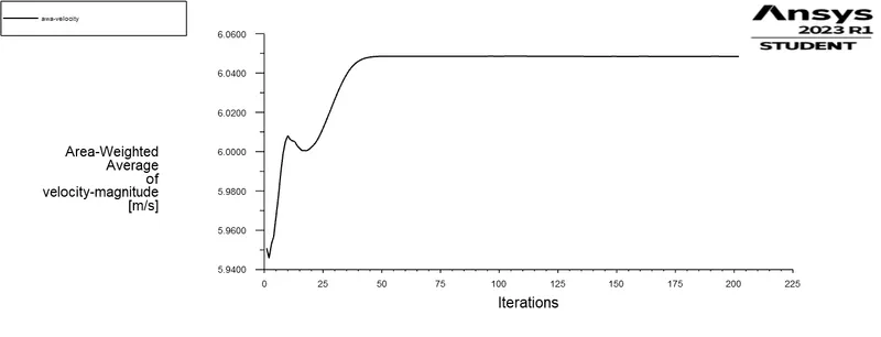 |
| Standard deviation of Temperature | 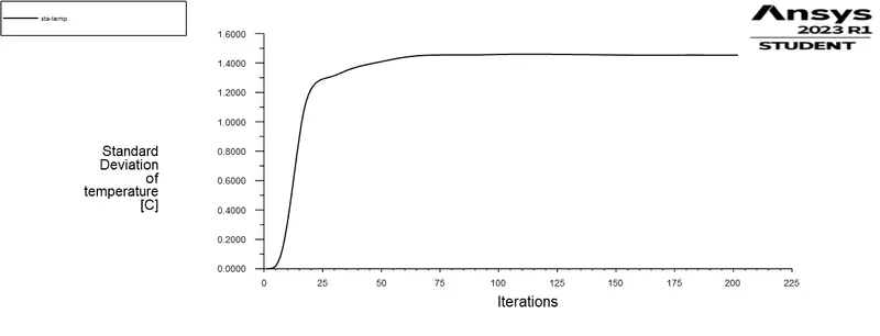 |
| Standard deviation of Velocity | 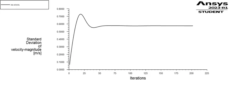 |
Contout plots
Case 2a
| Residuals | 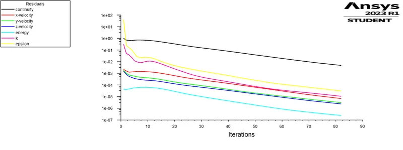 |
| Average outlet temperature | 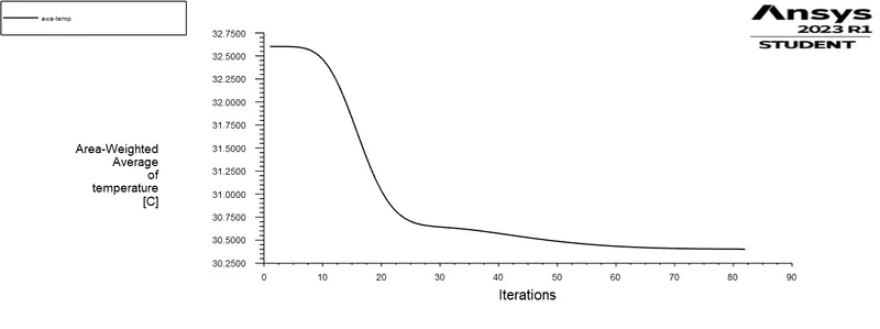 |
| Average outlet velocity | 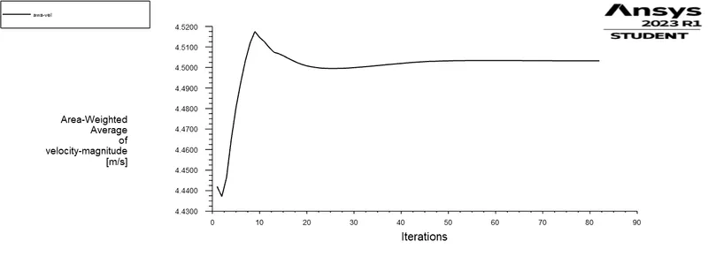 |
| Standard deviation of Temperature | 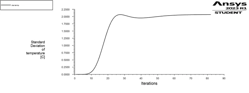 |
| Standard deviation of Velocity | 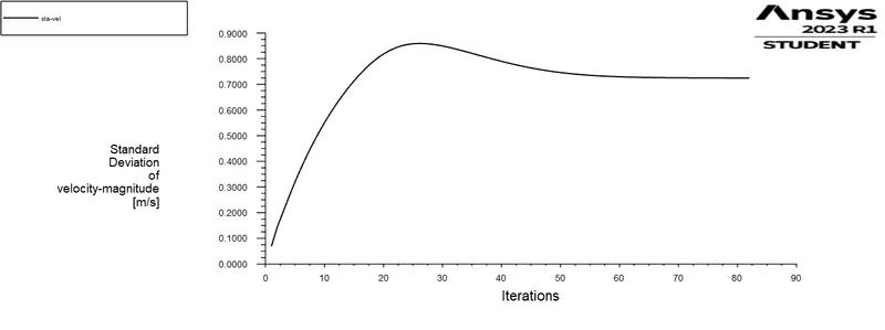 |
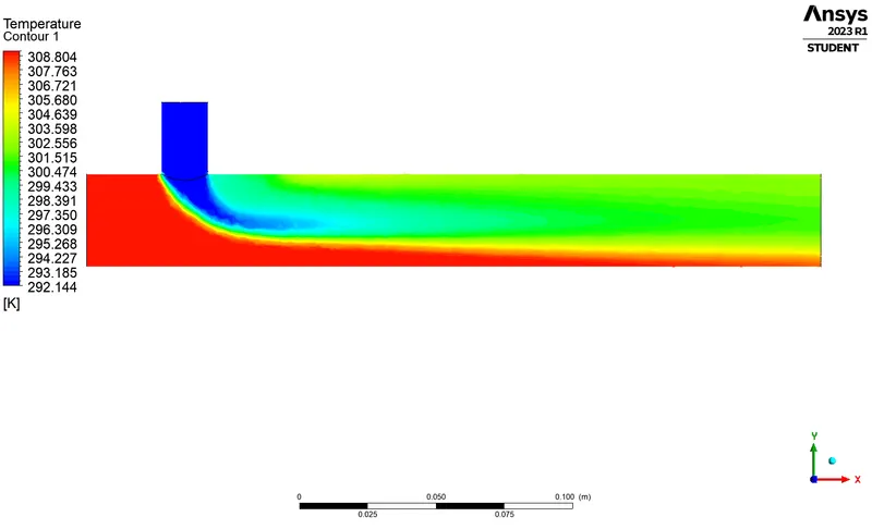
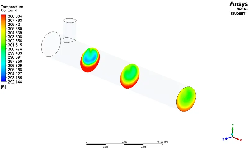
Contour plot
 s
s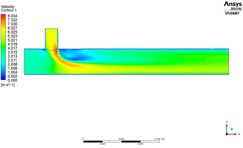
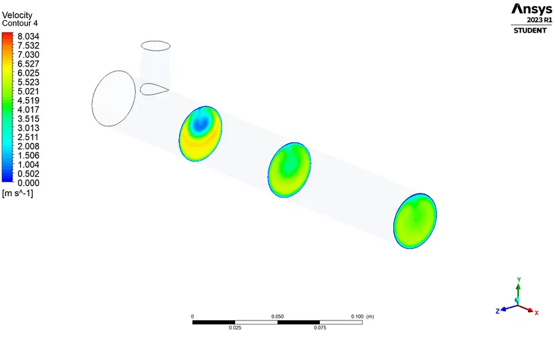
Case 2b
| Residuals | 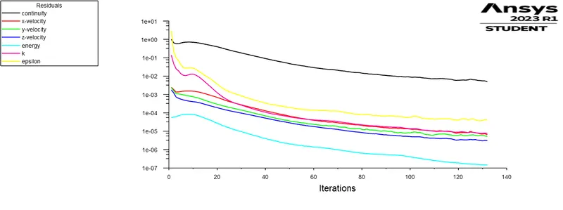 |
| Average outlet temperature | 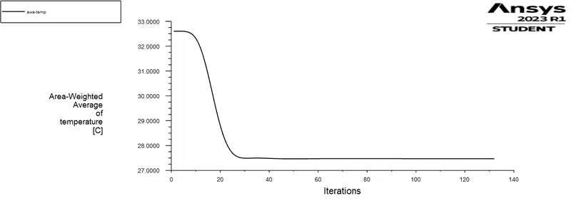 |
| Average outlet velocity | 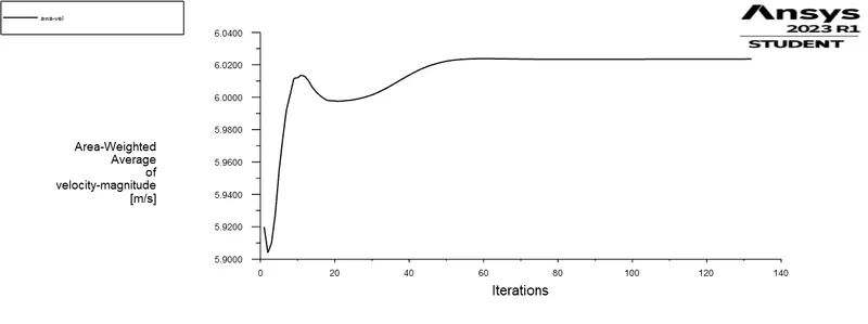 |
| Standard deviation of Temperature | 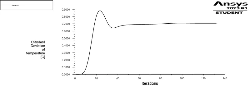 |
| Standard deviation of Velocity | 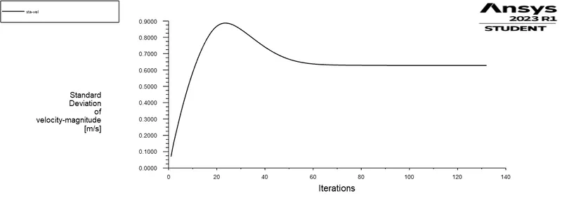 |
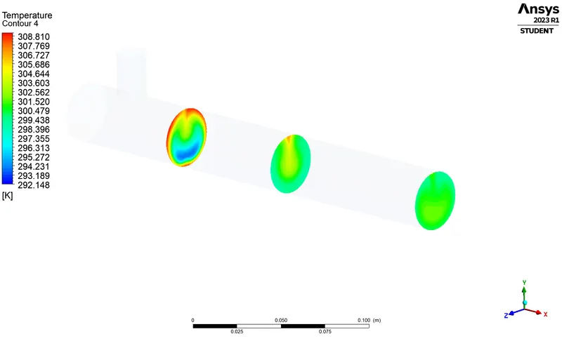
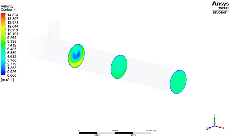
Contour plots
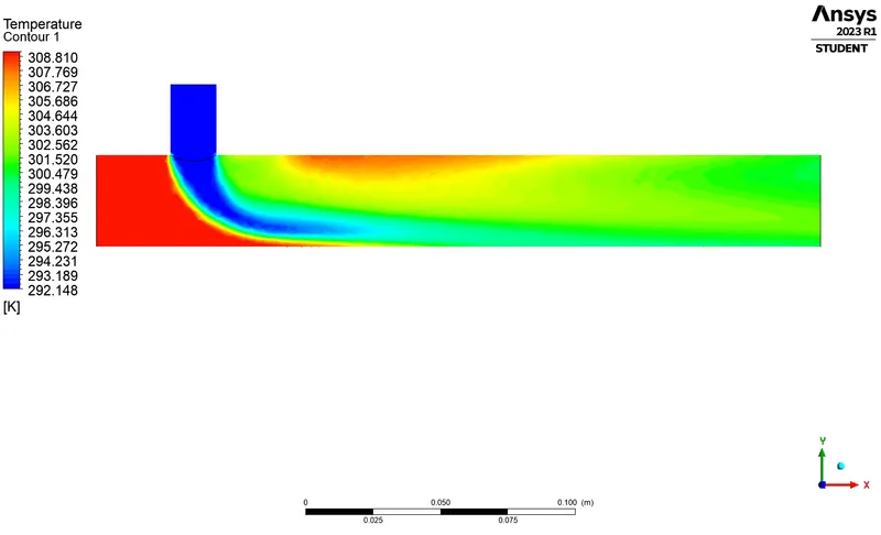
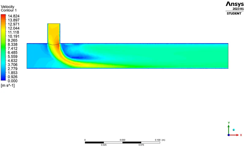
Effectiveness of Mixing
The high standard deviation implies better mixing. Observing the cases it shows that higher momentum ratio is giving lesser standard deviation
for cases 1a and 2a the SD is around 2 for Temperature.
But when Momentum ratio is 4 i.e., 1b and 2b standard deviation is less than the case 1a and 2a.
| Case | Average Temperature | Average Velocity | Standard deviation Temperature | Standard deviation Velocity |
| 1a | 30.337 | 4.5081 | 2.5641 | 0.64687 |
| 1b | 27.613 | 6.0484 | 1.4527 | 0.57547 |
| 2a | 30.403 | 4.5032 | 2.0693 | 0.7243 |
| 2b | 27.472 | 6.0236 | 0.70678 | 0.62787 |
The length does not create any change in temperature.
When looking at the contour plots it is seen that the uniformity of temperature is better for long tee.
Conclusion:
- K-epsilon model is selected over k-omega SST as the former gives better results when compared to analytical solution.
- Mesh independence test is performed for case 1a and the same mesh setting is used for other 3 cases.
- The velocity at the outlet is dependent on the Momentum ratio as we have seen in case 1b and case 2b.
- The effective mxing is obtained when the length of tee increased but it has no effect on temperature.