Week 7 - Simulation of a 1D Super-sonic nozzle flow simulation using Macormack Method
Simulation of a 1D Super-sonic nozzle flow simulation using Macormack Method
Aim: To simulate the isoentropic flow through a quasi 1D subsonic-supersonic nozzle using conservation and non-conservation forms of governing equation and solving them by MacCormack's method. investigating the difference of both forms of governing equation.
Objective: To obtain
- Steady-state distribution of primitive variables inside the nozzle
- Time-wise variation of the primitive variables
- Variation of Mass flow rate distribution inside the nozzle at different time steps during the time-marching process
- Comparison of Normalized mass flow rate distributions of both forms
- and Perform grid independence test
Subsonic-supersonic isoentropic flow: the problem here considered is steady, isoentropic flow through a convergent-divergent nozzle. The flow at the inlet to the nozzle comes from a reservoir and flow expands isoentropically at the nozzle exit.
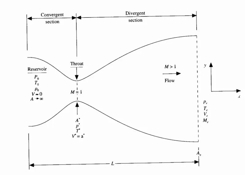
fig: schematic for subsonic-supersonic isoentropic flow (computational fluid dynamics by John D, Anderson jr)
The flow variable is represented using subscript 0 and e for reservoir and exit respectively. At the throat, variables are denoted by an asterisk.
For a nozzle with a specified area ratio, the pressure ratio drives the flow. It is the boundary condition applied to flow in the laboratory.
The problem is simplified to one-dimensional. Such simplification usually compromises the real physics of the flow. To ensure the governing equations are appropriate for quasi-one-dimensional flow, we have used integral forms of governing equations and resolved them into simpler forms.
Governing flow equations:
Non-conservation form
Continuity : `(del(rhoA))/(delt)+rhoA(delV)/(delx)+rhoV(delA)/(delx)+VA(delrho)/(delx) = 0`
Momentum : `rho(delV)/(delt)+rhoV(delV)/(delx) = -R(rho(delT)/(delx)+T(delrho)/(delx))`
Energy : `rhoc_v(delT)/(delt) + rhoVc_v(delT)/(delx) = -rhoRT[(delV)/(delx)+V(del(lnA))/(delx)]`
Conservation form
Continuity : `(del(rhoA))/(delt) + (del(rhoAV))/(delx) = 0`
Momentum : `(del(rhoAV))/(delt) + (del(rhoAV^2))/(delx) = -A(delp)/(delx)`
Energy : `(del[rho(e+V^2/2)A])/(delt) +(del[rho(e+V^2/2)AV])/(delx) = 0`
These are equations for quasi-one-dimensional flow in both non-conservation and conservation forms.
The above equations are in terms of dimensional variables. For non-dimesionsialising, we define the nondimensional temperature as`T' = T/T_0` and density as `rho' = rho/rho_0`.
dimensionless length `x' = x/L`
dimensionless velocity `V' = V/a_0`, where `a_0` is speed of sound denoted as `a_0 = sqrt(gammaRT_0)`
dimensionless time `t = t/(L/a_0)`
dimensionless area `A' = A/A^*`
substituting the dimensionless variables in the above equations we obtain the non dimensional equations
For non conservation form
Continuity : `(del(rho'A'))/(delt')=-rho'A'(delV')/(delx')-rho'V'(delA')/(delx')-V'A'(delrho')/(delx')`
Momentum : `(delV')/(delt') = -V'(delV')/(delx') -1/gamma((delT')/(delx') + (T')/(rho') (delrho')/(delx'))`
Energy : `(delT')/(delt') = -V'(delT')/(delx') - (gamma-1)T'[(delV')/(delx')+ V'(del(lnA'))/(delx')]`
for conservation form
Continuity : `(del(rho'A'))/(delt') + (del(rho'A'V'))/(delx') = 0`
Momentun : `(del(rho'A'V'))/(delt') + (del[rho'A'V'^2 + (1/gamma)p'A'])/(delx) = (1/gamma)p'(delA')/(delx')`
Energy : `(del[rho'((e')/(gamma-1)+gamma/2V'^2)A'])/(delt') + (del[rho'((e')/(gamma-1)+gamma/2V'^2)V'A' + p'A'V'])/(delx')`
further the conservation form is written in generic form by defining the solution vector U, the flux vector F, and the source term J.
`U_1 = rho'A'`
`U_2 = rho'A'V'`
`U_3 = rho'((e')/(gamma-1)+gamma/2V'^2)A'`
`F_1 = rho'A'V'`
`F_2 = rho'A'V'^2 + 1/gammap'A'`
`F_3 = rho'((e')/(gamma-1)+gamma/2V'^2)V'A'+p'A'V'`
`J_2 = 1/gammap'(delA')/(delx')`
these can be written as
`(delU_1)/(delt') = -(delF_1)/(delx')`
`(delU_2)/(delt') = -(delF_2)/(delx')+J_2`
`(delU_3)/(delt') = -(delF_3)/(delx')`
MacCormack's method is the finite difference method for hyperbolic partial differential equations.
In this method first, we solve the non-dimensional equation by forward difference scheme, update the values and then solve the same using the backward differencing. The first one is called the predictor step and later the corrector step. After the corrector step, we find the average time derivatives using both the corrector and predictor steps. then update the final solution.
for the calculation of the time step, we have used the CFL criterion for one-dimensional flow. `Deltat = C(Deltax)/(a+V)`, here a is local sonic velocity. local adaptive time control is implemented in each time step.
Matlab code
Main program
clear
close all
clc

%input parameters
%inputs
n = 31;
x = linspace(0,3,n);
dx = x(2) - x(1);
gamma = 1.4;
C= 0.5; %courant number
I = 1:n;

%Area profile
a = 1 + 2.2*(x-1.5).^2;
throat = find(a==1);

%number of time steps
nt = 1400;

[mass_c,p_c,v_c,T_c,rho_c,M_c] = Conservative(x,dx,n,nt,C);

[mass_nc,p_nc,v_nc,T_nc,rho_nc,M_nc] = Non_conservative(x,dx,n,nt,C);

[mass_a,p_a,T_a,rho_a,M_a] = Analytical(x,n);

figure(4)
plot(x,mass_nc,'linewidth',1.1)
hold on
plot(x,mass_c,'linewidth',1.1)
hold on
plot(x,mass_a,'--','linewidth',1.1,'color','k')
legend('non conservative','conservative','analytical')
ylabel('(rhoVA)/(rho_0a_0^*)')
xlabel('x/L')
title('comparison of mass flow rate in conservative and non conservative forms')
in the program, we have called three functions for conversation form, non-conservation form, and Analytical solution.
We have defined the number of grid points, the step size, constants in the program like gamma, and courant number.
Then we have plotted the comparison of mass flow for different forms of governing equations and analytical solutions.
In this program, we can change the number of nodes and time steps, and the courant number to obtain the results.
Function for Analytical solution
function [mass,pressure,temperature,density,mach_number] = Analytical(x,n)
I = 1:n;
gamma = 1.4;
rho_stag = 1;
temp_stag = 1;
m = 0;
a = 1 + 2.2*(x-1.5).^2;
b = a*-1;
at = (find(a==1)); %node of the throat

mach_number = zeros(1,n);
%finding the mach number at each point throughout the nozzle
%till the troat

for i = 1:at
    residual = 1;
    while residual  > 1e-9
        m = m + 1e-4;
        residual = ((1/m^2)*((2/(gamma+1))*(1+((gamma-1)/2)*m^2))^((gamma+1)/(gamma-1)))-a(i)^2;
    end
    mach_number(i) = m;
end

%from throat to exit
for i = at+1:n
    residual = 1;
    while residual > 1e-9
        m = m + 1e-4;
        residual = ((1/m^2)*((2/(gamma+1))*(1+((gamma-1)/2)*m^2))^((gamma+1)/(gamma-1)))-a(i)^2;
        residual = residual * -1;
    end
    mach_number(i) = m;
end

temperature = (1 + ((gamma-1)/2).*mach_number.^2).^(-1);
density = (1 + ((gamma-1)/2).*mach_number.^2).^((-1)/(gamma-1));
pressure = density.*temperature;
mass = density.*a.*mach_number.*sqrt(temperature);

figure1 = figure('position',[30,30,500,700]);
subplot(5,1,1)
plot(x,a,'b')
hold on
plot(x,b,'b')
hold on
plot([x(at) x(at)],[5,-5],'--','color','k')
title('Analytical solution')
subplot(5,1,2)
plot(x,mach_number,'k');
hold on
plot([0 x(at)],[mach_number(at) mach_number(at)],'--','color','k')
hold on
plot([x(at) x(at)], [0 mach_number(at)], '--', 'color','k')
hold on
plot([0 x(n)],[mach_number(n) mach_number(n)],'--','color','k')
yticks([0 1 mach_number(n)]);
yticklabels({'0',mach_number(at),'M_e'})
xlabel('x')
ylabel('Mach number')

subplot(5,1,3)
plot(x,pressure,'b');
hold on
plot([0 x(at)],[pressure(at) pressure(at)],'--','color','k')
hold on
plot([x(at) x(at)], [0 pressure(at)], '--', 'color','k')
hold on
plot([0 x(n)],[pressure(n) pressure(n)],'--','color','k')
yticks([0 pressure(n) pressure(at)]);
yticklabels({'0','p_e/p_0',pressure(at),'1'})
xlabel('x')
ylabel('pressure ratio')

subplot(5,1,4)
plot(x,temperature,'r');
hold on
plot([0 x(at)],[temperature(at) temperature(at)],'--','color','k')
hold on
plot([x(at) x(at)], [0 temperature(at)], '--', 'color','k')
hold on
plot([0 x(n)],[temperature(n) temperature(n)],'--','color','k')
yticks([0 temperature(n) temperature(at)]);
yticklabels({'0','T_e/T_0',temperature(at),'1'})
xlabel('x')
ylabel('Temperature ratio')

subplot(5,1,5)
plot(x,density,'g');
hold on
plot([0 x(at)],[density(at) density(at)],'--','color','k')
hold on
plot([x(at) x(at)], [0 density(at)], '--', 'color','k')
hold on
plot([0 x(n)],[density(n) density(n)],'--','color','k')
yticks([0 density(n) density(at)]);
yticklabels({'0','rho_e/rho_0',density(at),'1'})
xlabel('x')
ylabel('density ratio')

end
- The mach number variation is exclusively governed by the area ratio through the relation `(A/A^*)^2 = 1/M^2[(2/(gamma+1)(1+(gamma-1)/2M^2)]^((gamma+1)/(gamma-1))`
- variation of pressure, density and temperature as a function of Mach number is given by
- `p/p_0 = (1+(gamma-1)/2M^2)^(-gamma/(gamma-1)`
- `rho/rho_0 = (1+(gamma-1)/2M^2)^(-1/(gamma-1)`
- `T/T_0 = (1+(gamma-1)/2M^2)^(-1)`
- The mass flow rate is also calculated using density, area, temperature, and Mach number. All the variables are stored with _a.
Function for Conservation form
function [mass_c,p_c,v_c,T_c,rho_c,M_c] = Conservative(x,dx,n,nt,C)

gamma = 1.4;

%preallocating
rho = zeros(1,length(x));
T = zeros(1,length(x));
j2 = zeros(1,length(n)-2);
du1dt_p = zeros(1,length(n)-2);
du2dt_p = zeros(1,length(n)-2);
du3dt_p = zeros(1,length(n)-2);
du1dt_c = zeros(1,length(n)-2);
du2dt_c = zeros(1,length(n)-2);
du3dt_c = zeros(1,length(n)-2);
 rho_throat = zeros;
 p_throat = zeros;
 T_throat = zeros;
 M_throat = zeros;

%initial conditions
a = 1 + 2.2*(x-1.5).^2; %nozzle area
throat = find(a==1);

%density and temperature
for i = 1:length(x)
    if x(i)>=0 && x(i)<=0.5
        rho(i) = 1;
        T(i) =1;
    elseif x(i)>=0.5 && x(i)<=1.5
        rho(i) = 1.0 - 0.366*(x(i)-0.5);
        T(i) = 1.0 - 0.167*(x(i)-0.5);
    elseif x(i)>=1.5 && x(i)<=3
        rho(i) = 0.634 - 0.3879*(x(i)-1.5);
        T(i) = 0.833 - 0.3507*(x(i)-1.5);
    end
end

v = 0.59./(rho.*a); %velocity
p = rho.*T;

%initial solution vectors
u1 = rho.*a;
u2 = rho.*a.*v;
u3 = rho.*a.*((T./(gamma-1))+((gamma/2).*v.^2));

  rho_c = u1./a;                                    %density
  v_c = u2./u1;                                     %velocity
  T_c = (gamma-1)*((u3./u1) - (gamma/2).*v.^2);     %Temperature
  p_c = rho.*T;

%outer timeloop
for k = 1:nt

    %adaptive timestep control
    dt = min((C.*dx./(sqrt(T)+v)));

    u1_old = u1;
    u2_old = u2;
    u3_old = u3;

    %calculating the flux vectors
    f1 = u2;
    f2 = (u2.^2./u1) + ((gamma-1)/gamma)*(u3 - ((gamma/2)*u2.^2./u1));
    f3 = (gamma*u2.*u3./u1) - (gamma*(gamma-1)/2)*(u2.^3./u1.^2);

    %predictor method
    for j = 2:n-1
        %source term
        j2(j) = (1/gamma)*rho(j)*T(j)*(a(j+1)-a(j))/dx;

        %continuity
        du1dt_p(j) = -((f1(j+1) - f1(j))/dx );

        %momentum
        du2dt_p(j) = -((f2(j+1)-f2(j))/dx) + j2(j);

        %energy
        du3dt_p(j) = -((f3(j+1)-f3(j))/dx);

        %updating values
        u1(j) = u1_old(j) + du1dt_p(j)*dt;
        u2(j) = u2_old(j) + du2dt_p(j)*dt;
        u3(j) = u3_old(j) + du3dt_p(j)*dt;
    end


    %updating flux vectors
    f1 = u2;
    f2 = (u2.^2./u1) + ((gamma-1)/gamma)*(u3 - ((gamma/2)*u2.^2./u1));
    f3 = (gamma*u2.*u3./u1) - (gamma*(gamma-1)/2)*(u2.^3./u1.^2);

    %corrector method
        for j = 2:n-1

       %source term
        j2(j) = (1/gamma)*rho(j)*T(j)*(a(j)-a(j-1))/dx;

        %continuity
        du1dt_c(j) = -((f1(j) - f1(j-1))/dx );

        %momentum
        du2dt_c(j) = -((f2(j)-f2(j-1))/dx) + j2(j);

        %energy
        du3dt_c(j) = -((f3(j)-f3(j-1))/dx);
        end

    %computing the time average derivative
    du1dt = 0.5*(du1dt_p + du1dt_c);
    du2dt = 0.5*(du2dt_p + du2dt_c);
    du3dt = 0.5*(du3dt_p + du3dt_c);

    %final solution update
    for i = 2:n-1
        u1(i) = u1_old(i) + du1dt(i)*dt;
        u2(i) = u2_old(i) + du2dt(i)*dt;
        u3(i) = u3_old(i) + du3dt(i)*dt;
    end

  %boundary conditions

  %inlet
  u1(1) = rho(1).*a(1);
  u2(1) = 2*u2(2) - u2(3);
  v(1) = u2(1)/u1(1);
  u3(1) = u1(1) * ((T(1)/(gamma-1))+(gamma/2)*v(1)^2);

  %outlet
  u1(n) = 2*u1(n-1) - u1(n-2);
  u2(n) = 2*u2(n-1) - u2(n-2);
  u3(n) = 2*u3(n-1) - u3(n-2);

  %calculating the primitive variables
  rho = u1./a;                                    %density
  v = u2./u1;                                     %velocity
  T = (gamma-1)*((u3./u1) - (gamma/2).*v.^2);     %Temperature
  p = rho.*T;                                     %pressure

  mass_c = (rho.*a.*v);
  %mach number
  M_c = v./(sqrt(T));

  %variation at throat
    rho_throat(k) = rho(throat);
    T_throat(k) = T(throat);
    p_throat(k) = p(throat);
    M_throat(k) = M_c(throat);
    mass_nc = (rho.*a.*v);

  figure(5)
    if k == 50
        plot(x,mass_c,'k','linewidth',1.1)
        hold on
    elseif k == 100
        plot(x,mass_c,'b','linewidth',1.1)
        hold on
    elseif k == 200
        plot(x,mass_c,'g','linewidth',1.1)
        hold on
    elseif k == 400
        plot(x,mass_c,'m','linewidth',1.1)
        hold on
    elseif k == 800
        plot(x,mass_c,'c','linewidth',1.1)
        hold on
    elseif k == nt
        plot(x,mass_c,'r','linewidth',1.1)
        title('variation of mass flow at different times for conservative form')
        xlabel('x/L')
        ylabel('(rhoVA)/(rho_0a_0^*)')
        legend('50th timestep','100th timestep','200th timestep','400th timestep','800th timestep','1400th timestep')
        hold off
    end
end
%mass
mass_c = (rho.*a.*v);


   nmtsp = linspace(1,nt,nt);

   figure(6)
   subplot(4,1,1)
   plot(nmtsp,rho_throat,'color','k')
   title('Time variations of the density, temperature, pressure and mach number at the nozzle throat for conservative form')
   ylabel('rho/rho_0')
   subplot(4,1,2)
   plot(nmtsp,T_throat,'color','k')
   ylabel('T/T_0')
   subplot(4,1,3)
   plot(nmtsp,p_throat,'color','k')
   ylabel('p/p_0')
   subplot(4,1,4)
   plot(nmtsp,M_throat,'color','k')
   ylabel('M')
   xlabel('Number of time steps')
end
- this function is written for solving the nondimensional form of the conservation equation.
- Initial conditions for conservation equations are
- `rho' = 1.0` and `T' = 1.0` for `0<=x'<=0.5`
- `rho' = 1.0 - 0.366(x'-0.5)_` and `T' = = 1.0 - 0.167(x'-0.5)` for `0.5<=x'<=1.5`
- `rho = 0.634 - 0.3879(x'-1.5)` and `T' = 0.833 - 0.3507(x'-1.5)` for `1.5<=x'<=3.5`
- and velocity `V' = U_2/(rho'A')` = `0.59/(rho'A')`
- from these the initial values of solution vectors are obtained by substituting in
- `U_1 = rho'A'`
- `U_2 = rho'A'V'`
- `U_3 = rho'((e')/(gamma-1)+gamma/2V'^2)A'`
- Using the initial values of u1 u2 and u3 fluxes are calculated.
- Using for loop for time step calculation and for loop for predictor and corrector step the values are calculated iteratively.
- then the primitive variables and calculated along with the mass flow rate.
- to study the time variation of the mass flow rate the value is calculated at the throat for different time steps and the same is plotted.
Function for non-conservation form
function [mass_nc,p,v,T,rho,M] = Non_conservative(x,dx,n,nt,C)

gamma = 1.4;

%initial profiles
rho = 1 - 0.3146*x;
T = 1 - 0.2314*x;
v = (0.1 + 1.09*x).*T.^0.5;
a = 1 + 2.2*(x-1.5).^2;
throat = find(a==1);


%preallocating
 dTdt_p = zeros(1,length(n));
 dvdt_p = zeros(1,length(n));
 drhodt_p = zeros(1,length(n));
 dTdt_c = zeros(1,length(n));
 dvdt_c = zeros(1,length(n));
 drhodt_c = zeros(1,length(n));
 rho_throat = zeros;
 p_throat = zeros;
 T_throat = zeros;
 M_throat = zeros;


%time loop
 for k = 1:nt
    rho_old = rho;
    v_old = v;
    T_old = T;

    %adaptive time control
    dt = min((C*dx./(sqrt(T)+v)));

    %predictor method
    for j = 2:n-1
        dvdx = (v(j+1) - v(j))/dx;
        drhodx = (rho(j+1) - rho(j))/dx;
        dTdx = (T(j+1) - T(j))/dx;
        dlogadx = (log(a(j+1)) - log(a(j)))/dx;

        %continuity equation
        drhodt_p(j) = -rho(j)*dvdx - rho(j)*v(j)*dlogadx - v(j)*drhodx;
        %momentum equation
        dvdt_p(j) = -v(j)*dvdx - (1/gamma)*(dTdx + (T(j)/rho(j))*drhodx);
        %energy equation
        dTdt_p(j) = -v(j)*dTdx - (gamma-1)*T(j)*(dvdx + v(j)*dlogadx);

        %updating values
        rho(j) = rho(j) + drhodt_p(j)*dt;
        v(j) = v(j) + dvdt_p(j)*dt;
        T(j) = T(j) + dTdt_p(j)*dt;
    end


    %corrector step
    for j = 2:n-1
        dvdx = (v(j) - v(j-1))/dx;
        drhodx = (rho(j) - rho(j-1))/dx;
        dTdx = (T(j) - T(j-1))/dx;
        dlogadx = (log(a(j)) - log(a(j-1)))/dx;

        %continuity equation
        drhodt_c(j) = -rho(j)*dvdx - rho(j)*v(j)*dlogadx - v(j)*drhodx;
        %momentum equation
        dvdt_c(j) = -v(j)*dvdx - (1/gamma)*(dTdx + (T(j)/rho(j))*drhodx);
        %energy equation
        dTdt_c(j) = -v(j)*dTdx - (gamma-1)*T(j)*(dvdx + v(j)*dlogadx);
    end

    %computing the time average derivative
    drhodt = 0.5*(drhodt_p + drhodt_c);
    dvdt = 0.5*(dvdt_p + dvdt_c);
    dTdt = 0.5 * (dTdt_p + dTdt_c);

    %final solutionn update
    for i = 2:n-1
        rho(i) = rho_old(i) + drhodt(i)*dt;
        v(i) = v_old(i) + dvdt(i)*dt;
        T(i) = T_old(i) + dTdt(i)*dt;
    end

    %boundary values
    %inlet
    v(1) = 2*v(2)-v(3);

    %outlet
    v(n) = 2*v(n-1)-v(n-2);
    rho(n) = 2*rho(n-1) - rho(n-2);
    T(n) = 2*T(n-1) - T(n-2);

    p = rho.*T;
    M = v./sqrt(T);
    %variation at throat
    rho_throat(k) = rho(throat);
    T_throat(k) = T(throat);
    p_throat(k) = p(throat);
    M_throat(k) = M(throat);
    mass_nc = (rho.*a.*v);

    figure(2)
    if k == 50
        plot(x,mass_nc,'k','linewidth',1.1)
        hold on
    elseif k == 100
        plot(x,mass_nc,'b','linewidth',1.1)
        hold on
    elseif k == 200
        plot(x,mass_nc,'g','linewidth',1.1)
        hold on
    elseif k == 400
        plot(x,mass_nc,'m','linewidth',1.1)
        hold on
    elseif k == 800
        plot(x,mass_nc,'c','linewidth',1.1)
        hold on
    elseif k == 1400
        plot(x,mass_nc,'r','linewidth',1.1)
        title('variation of mass flow at different times for non conservative form')
        xlabel('x/L')
        ylabel('(rhoVA)/(rho_0a_0^*)')
        legend('50th timestep','100th timestep','200th timestep','400th timestep','800th timestep','1400th timestep')
    end

end

   nmtsp = linspace(1,nt,nt);

   figure1 = figure('position',[30,30,500,700]);
   subplot(4,1,1)
   plot(nmtsp,rho_throat,'color','k')
   title('Time variations of the density, temperature, pressure and mach number at the nozzle throat for non conservative form')
   ylabel('rho/rho_0')
   subplot(4,1,2)
   plot(nmtsp,T_throat,'color','k')
   ylabel('T/T_0')
   subplot(4,1,3)
   plot(nmtsp,p_throat,'color','k')
   ylabel('p/p_0')
   subplot(4,1,4)
   plot(nmtsp,M_throat,'color','k')
   ylabel('M')
   xlabel('Number of time steps')

   %non dimensional mass flow
   mass_nc = (rho.*a.*v);

end
- The initial profile is defined for non-conservative form
- rho = 1 - 0.3146*x;
T = 1 - 0.2314*x;
v = (0.1 + 1.09*x).*T.^0.5;
a = 1 + 2.2*(x-1.5).^2; - after the predictor and corrector step the boundary conditions are applied and the primitive variables are calculated.
- the mass flow rate at different time steps are plotted using if loop
- to study the time-wise variation the values at the throat are selected and stored for every time step and plotted.
Outputs
Timewise variation of the primitive variables for different forms of governing equation.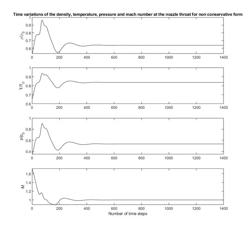
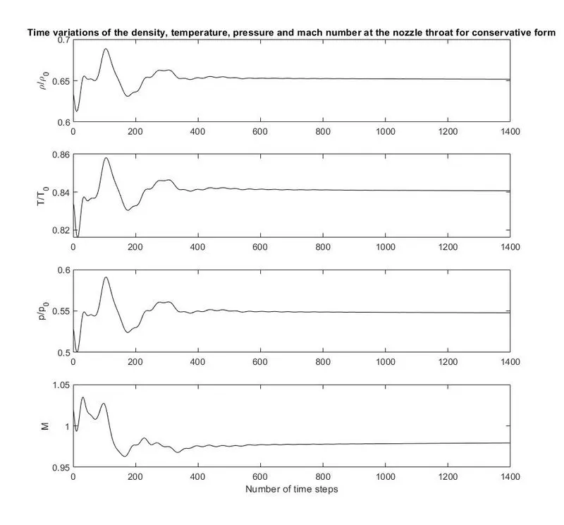
From the graphs, we can observe that the steady-state has been achieved after particular timesteps and calculation can be stopped. the x-axis is essentially the time. After some time steps the values stay flat and do not change it indicated the absence of artificial viscosity.
Initially, the values oscillate but later the values achieved a steady state.
Mass flow rates at different time marching steps
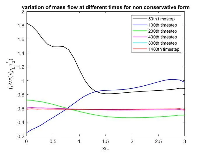
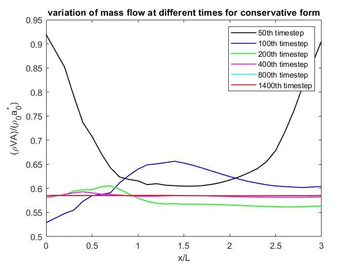
Here the non-dimensional mass flow is plotted as a function of non-dimensional length through the nozzle. when you observe the line for 50th and 100 timesteps, the mass flow has changed radically due to transient variation of the flow field variables. After the 200th time step the values being to stabilize and after the 800th time step, the values became stable.
Normalized mass flow for both conservative and nonconservative forms
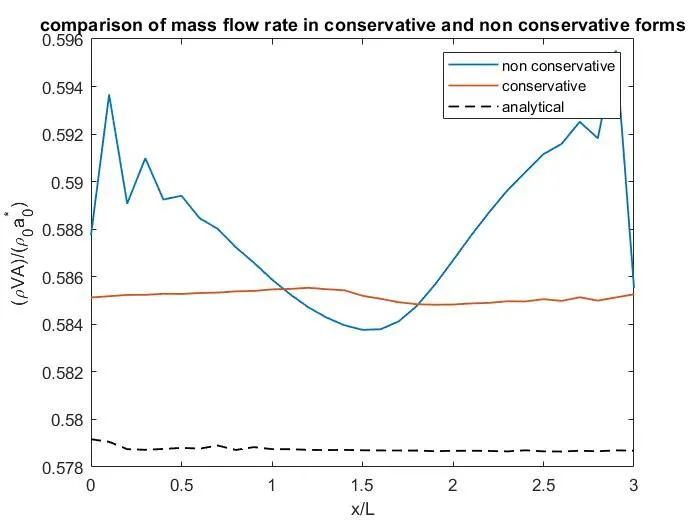
From the plot of mass flow rate, the conservative form seems to give more satisfactory results than non-conservative, which has variations in the inflow and outflow boundaries. The conservative form is closer to the exact analytical solution.
Grid independence test

Up to 3 decimals, the grid of 31 points seems to have good results with analytical solutions for non-conservative form.
for the conservative form when we look at the 61 points data for Mach number, the results are better for 61 compared to 31 grid points. so we can say it is grid-independent at 61 points for conservative form.
Conclusion
- The conservative form of equations has yielded better mass flow distribution. And seems to conserve mass better than the non-conservative form of the equation.
- When we look at the grid independence data the non-conservative form has given primitive variables closer to the exact analytical solution than another form. For example, the Mach number at 31 grid points is closer to the analytical solution by the non-conservative form than the conservative form.
- there is no clear superiority as the conservative form conserves the mass flow distribution but the non-conservative form yield better primitive variable results.
- When we look at the easiness of setting up and writing code for a solution, the non-conservative form fared better than another form.