Objective:
We have created two versions of the mixing tee. One of them is longer than the other. Our objective is to set up steady-state simulations to compare the mixing effectiveness when the hot inlet temperature is 360C & the Cold inlet is at 190C.
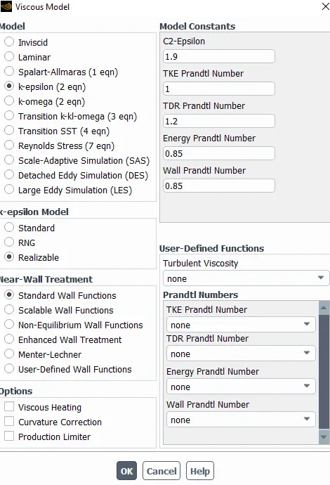
Using the k-epsilon and k-omega SST model for the first case and based on your judgment use the more suitable model for further cases. Giving the reason for choosing a suitable model is compulsory.
- Case 1
- Short mixing tee with a hot inlet velocity of 3m/s.
- Momentum ratio of 2, 4.
- Case 2
- Long mixing tee with a hot inlet velocity of 3m/s.
- Momentum ratio of 2, 4.
Momentum ratio = velocity at cold inlet / velocity at hot inlet
In a table, compare the following values from the 2 cases.
- Cell count
- Average outlet temperature
- Number of iterations for convergence
Expected results:
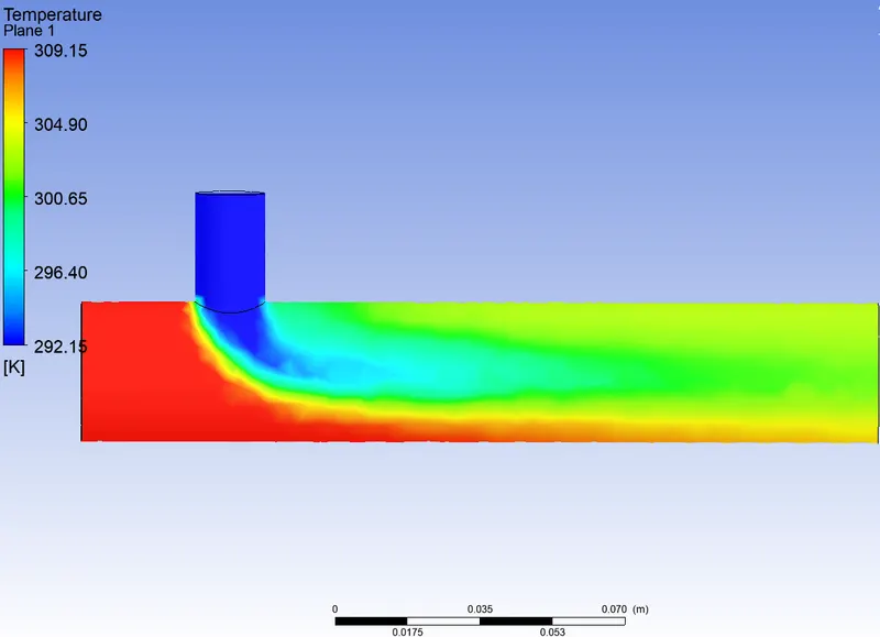
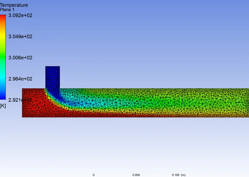
- Velocity and temperature contour plots on the cut planes along and across the pipe.
- Velocity and temperature line plots along and across the length of the pipe.
- Perform Mesh independent study for any one case.
- Discuss the effect of length and momentum ratio on results.
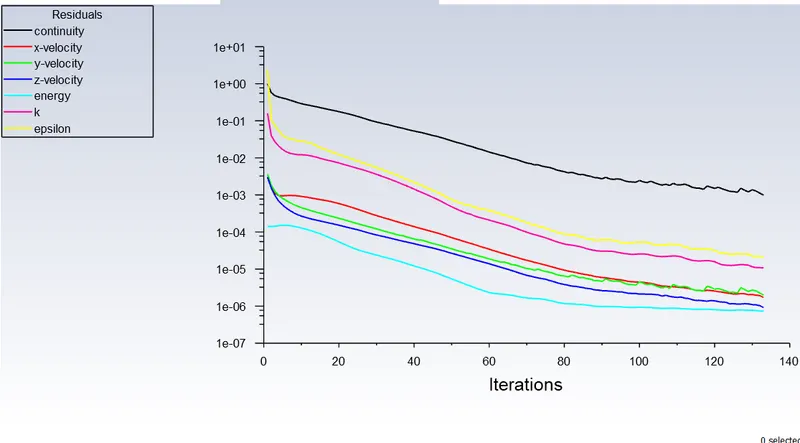
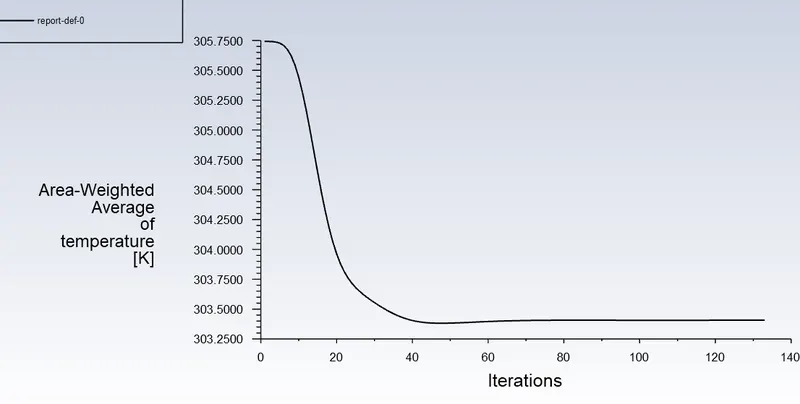
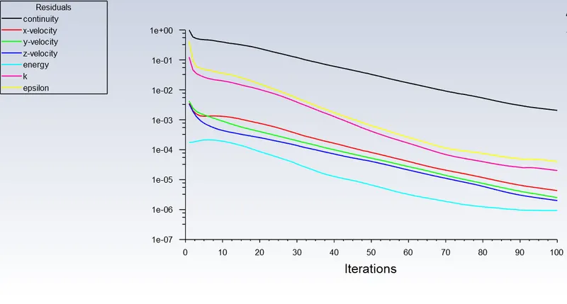
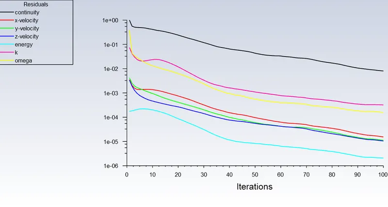
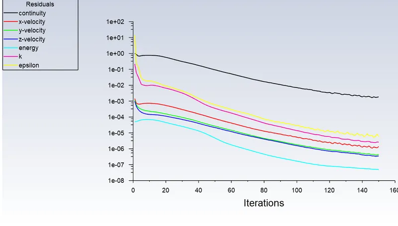
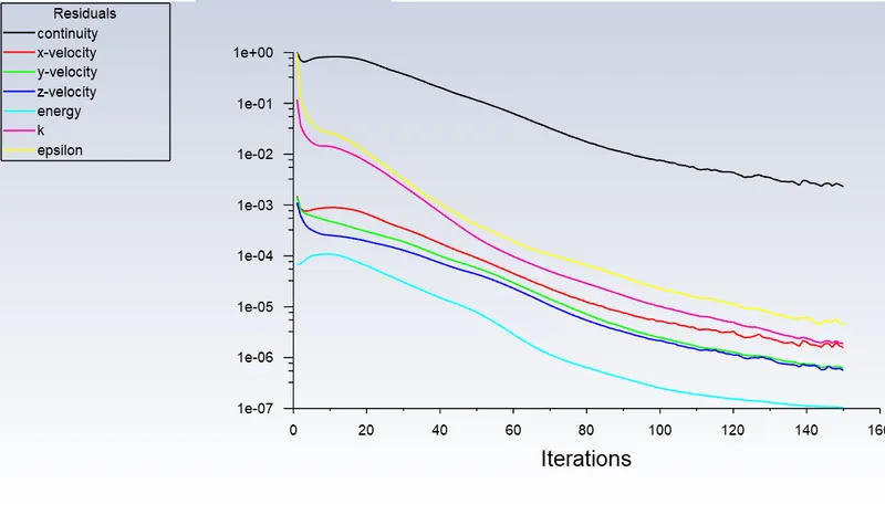
For each simulation, you need to show the convergence plot
Reference Research paper:- https://www.sciencedirect.com/science/article/pii/S0029549309005676
[Note - It is just a reference research paper, those who do not have access to this paper can use any other research paper. Try to imitate the results from this paper, even if answers don't match]
Reference Formulas:-
Solution:
CFD modeling of a mixing tee that is often found in the industry. Traditional simulation is validated against experiment, as well as a new commercially available method that offers the possibility of substantial solution time reduction. In fact, the new method is shown to give accurate results in a much shorter computer time than the traditional analysis, allowing a much more rapid turnaround of difficult problems such as the turbulent mixing behavior of industrial mixing tees.
When there is a large temperature difference between two fluid streams, large temperature fluctuations can occur, which can lead to thermal fatigue of the piping system, even at “steady-state” bulk flow conditions. Advanced CFD modeling is capable of predicting these fluid temperature fluctuations at the mix point, as well as characterizing the corresponding temperature variations in the pipe wall itself. Specifically, large eddy simulation (LES) is required to capture the time-varying turbulent behavior at the mix point, which is significantly more time and resource-intensive than traditional two-parameter (e.g. k-e and k-w) Reynolds Averaged Navier-Stokes (RANS) simulation which is the workhorse of most industrial CFD simulation. In the first part of this twin blog, both the traditional LES approach and a new hybrid RANS-LES method are used to predict the mixing of the two fluid streams and the results are compared with test data reported in the literature for validation purposes. The new hybrid model is termed stress-blended eddy simulation (SBES) and has recently been included in the commercial software ANSYS/Fluent. SBES retains most of the fidelity of the traditional LES approach in a fraction of the time for typical problems. The SBES approach is then used in Part 2 as part of an actual industrial application to predict temperature fluctuations in a mixing tee. The simulation is used to determine the length of the thermal sleeve required to protect the pipe from thermal fatigue.
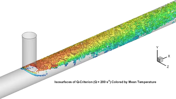
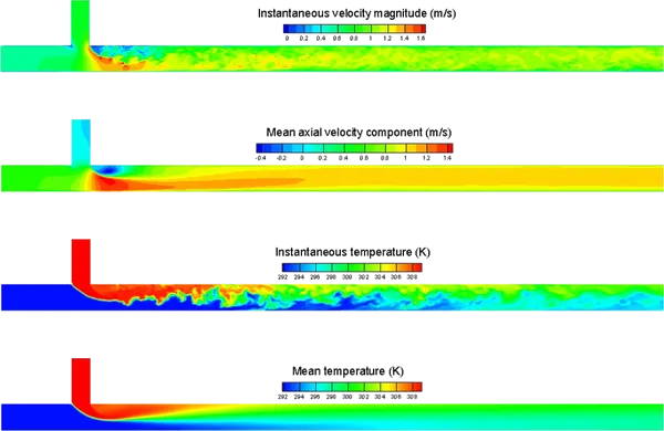
Turbulence is characterized by eddies with different space and time scales. In LES, large eddies are resolved directly, while small eddies are modeled using a subgrid model. LES requires significantly finer meshes and a smaller time step than those for a RANS model. SBES is a hybrid RANS-LES turbulence model, in which the boundary layer is modeled using an unsteady RANS model, while the LES model is applied to the core turbulent region where large turbulence scales play a dominant role. As such, SBES allows a coarser mesh and a larger time step than LES does.
The predicted time-averaged axial velocity component (u) and vertical velocity component (v) compare satisfactorily with the test data. The predicted fluctuations of the velocity components are also in good agreement with the measurements for both the LES and SBES simulations. It is whorth noting that the SBES simulation takes a much shorter time to solve than the LES simulation for the same basic results.
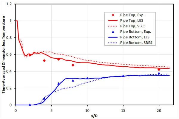
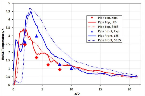
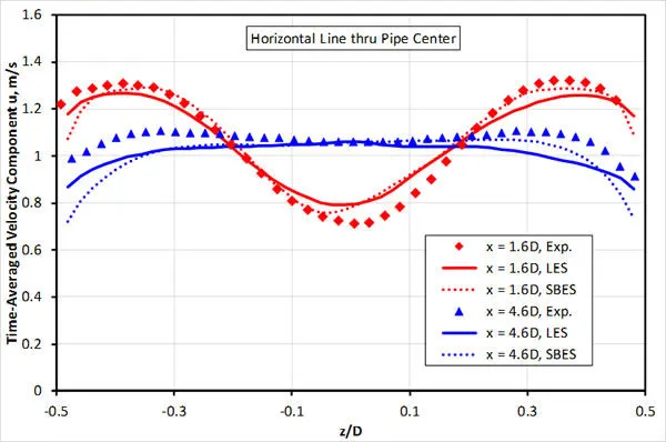
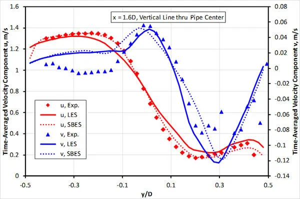
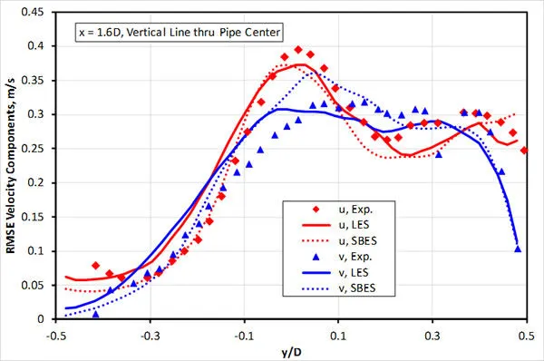
The model predictions show that the results from both the LES and SBES models are in excellent agreement with the measurements of the time-averaged and RMSE temperature and velocity components of the flow in a mixing tee. The SBES model can predict turbulent flow structures in the thermal mixing process. Since the SBES model requires a much lower computational cost and provides a faster turn-around of difficult problems than the LES model does, this approach will be used in Part 2 to predict temperature fluctuations in a mixing tee, which blends light gas oil with a recycled gas, to determine the length of a thermal sleeve which is used to protect the pressure boundary piping.
And the next thing we are going to do is to perform a mixing tee flow simulation where we get the idea of how this flow analysis works in CFD packages at the industrial level.
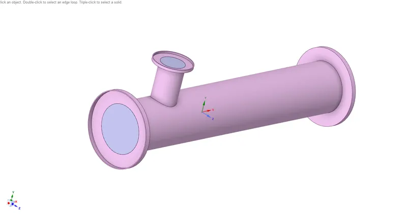
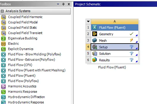
The CFD package that we are going to use is ANSYS-FLuent. And moreover, we are going to perform a simulation of 2 types of mixing tee.
1. Short Mixing tee
2. Long Mixing tee.
The files are already present in SLDPRT and STEP format. so we can download extract the same in the Ansys fluent. This is a Steady-state simulation with the comparison of mixing effectiveness at the Hot inlet 36C and cold outlet of 19C.
Short Mixing tee case -1
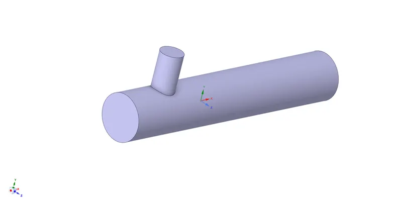
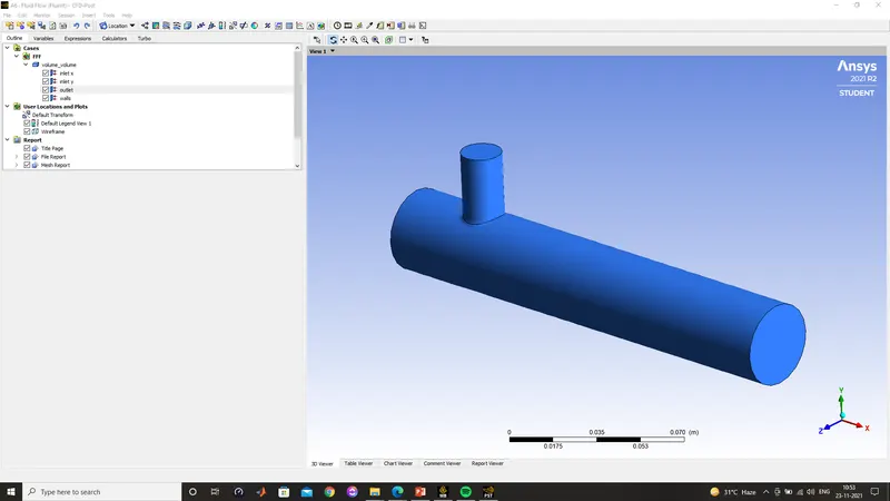
So first we are going to take a short mixing tee for simulation and here we extract and import the STEP file to Ansys-fluent. And the imported file is run in space claim, which is again an in-build CAD clean-up software in Ansys -Fluent. This is how we it looks like in the space claim. Although the steps to reach the solutions are the same only varies with grid dependencies test and variable momentum ratio test for both short and long mixing tee.
The above model is more modified to simpler channel flow where we ignore the thickness of the geometry and extract the volume alone from it. which makes us interested only in channel flow across the inlets and outlet. And assuming there's no heat flux running on the channel that may or may not affect the flow and the transfer of the heat.
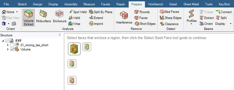
the following is the way we do it in the space claim. The steps involved are quite simple.
Prepare > Volume extract > select the faces > Ok
right-click on the volume in the tree and suppress the physics so that the whole unextracted body won't be coming in while going in for the mesh generation.
moving on to the mesh section where we generate mesh across the whole geometry. The following are the ways we can go to mesh tools. we have 5 sections here and this is how we perform all the simulations and validate our results with experimental data.
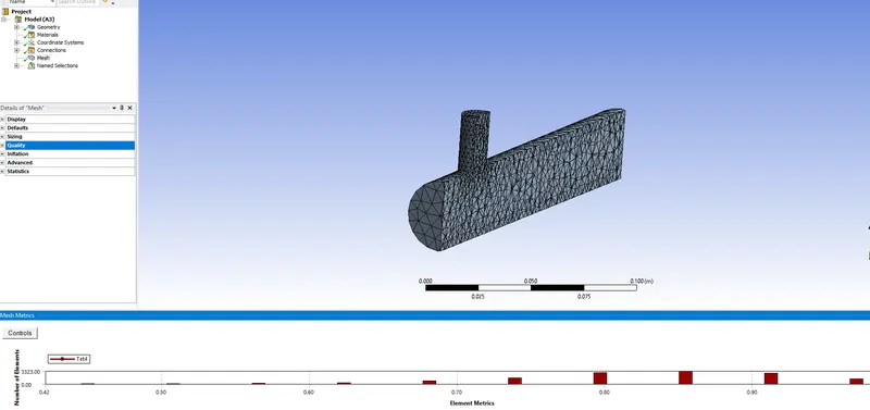
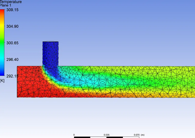
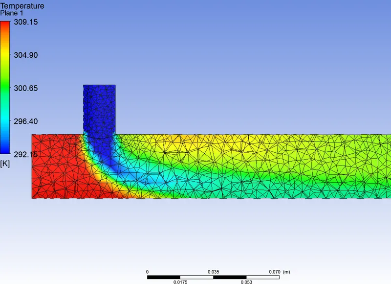
this is what mesh tools look like while we are about to generate the mesh. Here the idea is to just generate mesh along the surface where we have different grid dependencies for the geometry. The finer the mesh the more it takes to run the simulation. But here we see how it depends on different grid scaling.
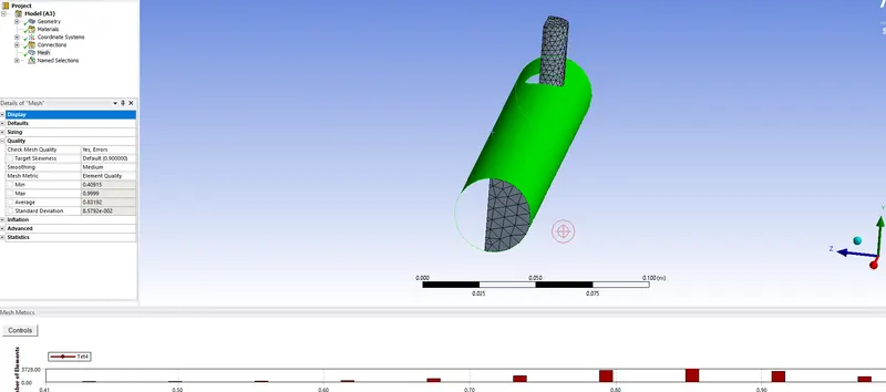
we sliced it in half to see the mesh inside of the geometry. Before hitting for the GENERATE MESH we are going to name the inlets, walls, and outlets.
and then we are going to hit generate the mesh. then later on we can change the quality of the mesh required to have a variety of grid dependencies.
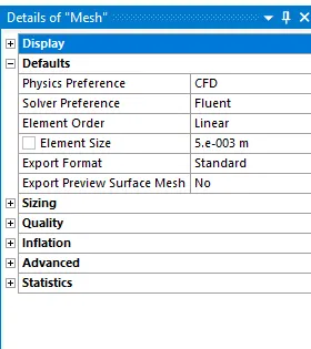
here at the quality mesh, we are going to perform a quality of the mesh by changing the values and changing the element size. The finer the mesh the longer it's going to take simulations to run and the more accurate the results will be.
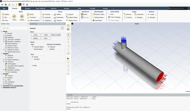
The next step is to run the simulation in the setup section where we can monitor the results too. This is the simulations part and next will post-processing the results.
Here we can decide, according to our system performance, whether we want to run parallel simulation or series. the dialogue box introduced here is the idea of what type simulation should be run. According to our processor, we can select how many processor to run.
before we move on to a different section for the simulations to run we have to perform our mesh quality check.
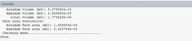
This is a console that gives you information about simulation and the features that you run here. It also represents the quality analysis for the mesh which affects the simulations partly. so we check for the quality and this is what shows us that the meshing check is done.
Now we have to divide this into 2 sections where we are going to add values to the simulations. so there is Physics and Solutions. In physics, we are going to define the boundary conditions and add wall functions which is the standard wall function here.
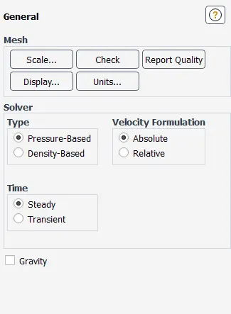
these are the following features that fluent provides for the simulation part in the physics section. So first we need to decide what kind of solver we are here going to use. since it's a simple incompressible flow we are going to select pressure-based steady-state simulations. With that, we are going to select the k-epsilon turbulence modeling with standard wall functions. This is how we are going to assign values to it.
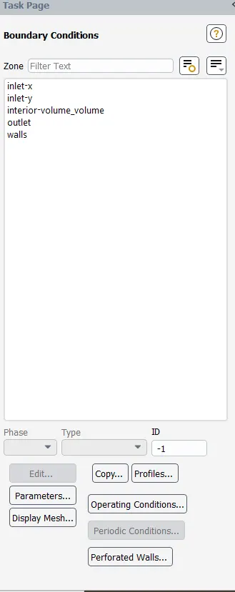
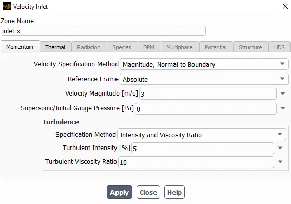
and we are going to assign boundary conditions under the boundaries section. and this how it looks like. The momentum ratio here will be taken as 2. So by formula, the inlet velocity of cold temperature will be 6ms-1.
with momentum ratio 4, the inlet velocity of cold temperature will be 12ms-1.
with momentum ratio 2, in long mixing tee, the inlet velocity of cold temperature will be 6ms-1.
with momentum ratio 4, in a long mixing tee, the inlet velocity of cold temperature will be 12ms-1.
and then by editing each boundary value you can assign their inlet and pressure outlet conditions.
This was the physics part and now we are moving on to the part of the solution where we spectate results while running the simulations. The solution section looks like this.
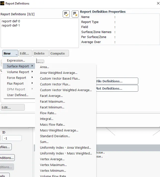
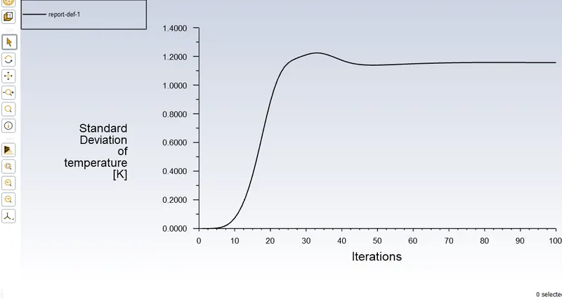
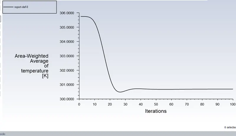
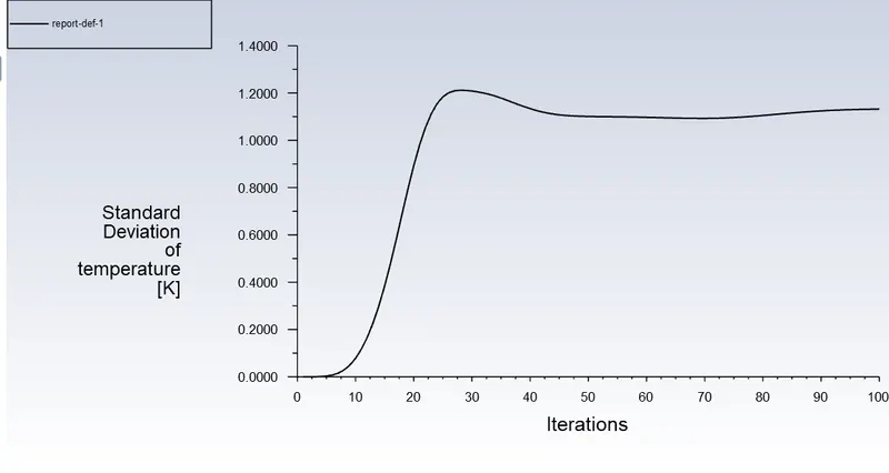
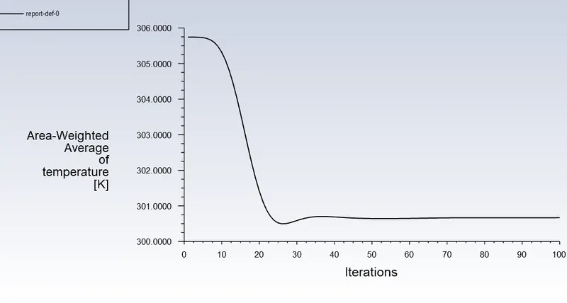
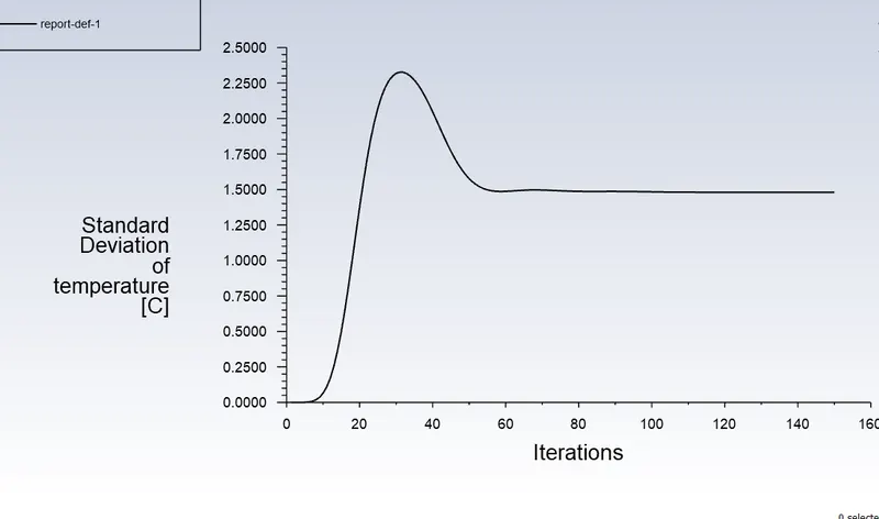
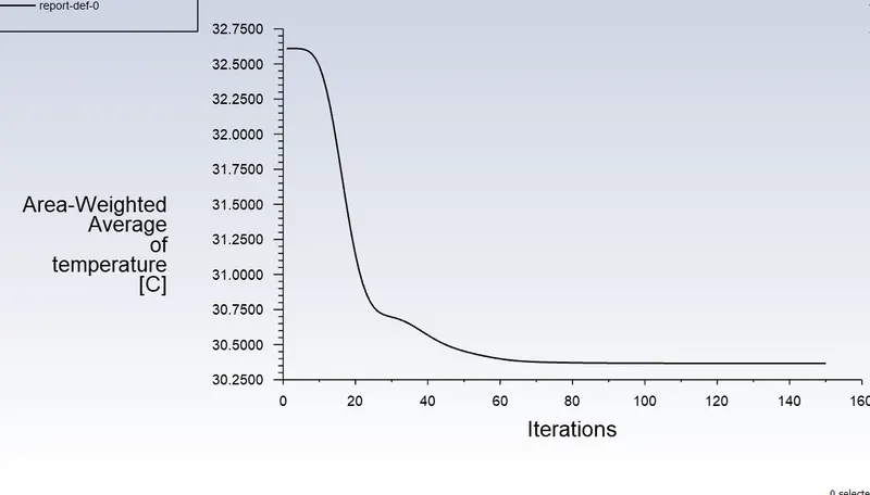
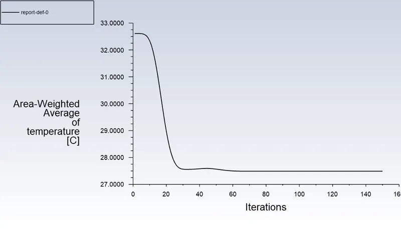
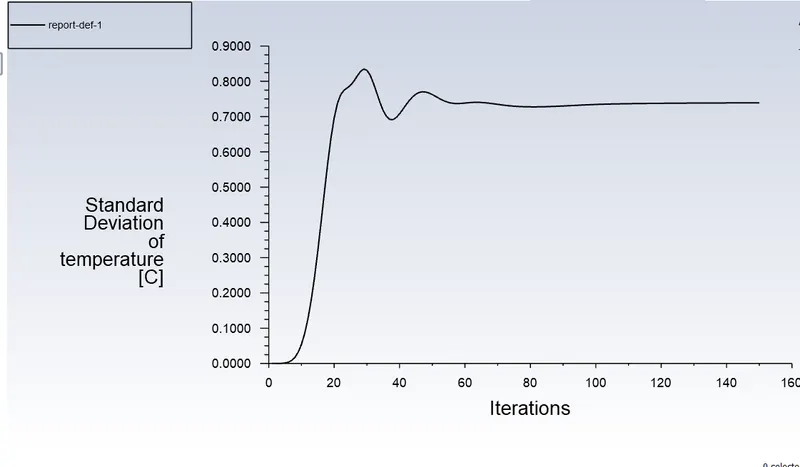
before we initialize the solutions we are going to be displaying some results and for that, we have a feature called definitions under REPORTS. This is how we assign the display reports. We are more interested in the outlet. So for that, we are going to see the average surface area of temperature and standard deviation of temperature at the outlet.
Here we select area-weighted average and standard deviation.
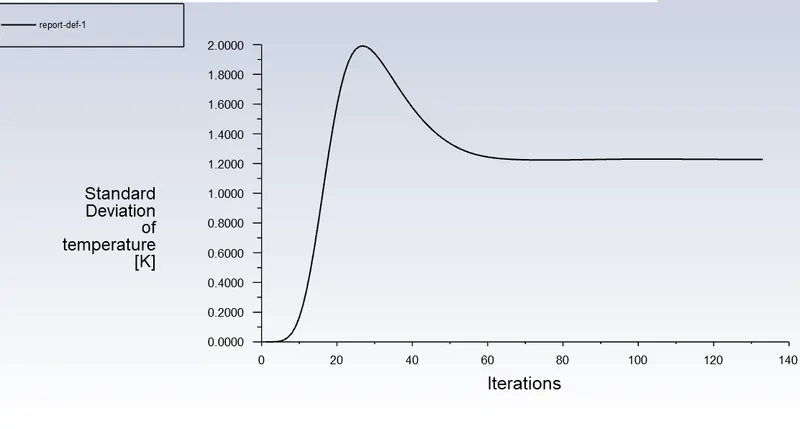
We hit initialize = 0 and then the solution icon to get the plots. Below are the results we tallied for different cases such as:
1. momentum ratio of 2, in short, mixing tee
2. momentum ratio of 4, in short, mixing tee
3. momentum ratio of 2, in a long mixing tee
4. momentum ratio of 4, in a long mixing tee
Results:
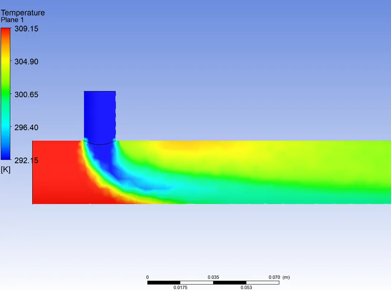
case 1:
case 2:
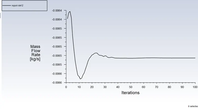
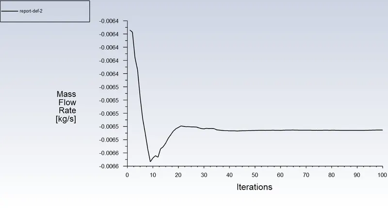
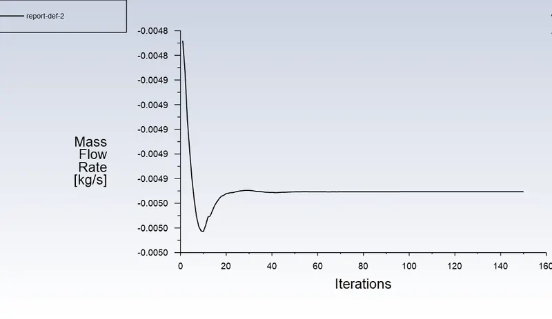
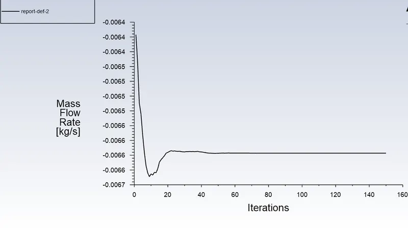
The mass flow rate is 0.0064 at its peak when running its iterations between 0 to 10. At, approximately around the 38th iteration the solution reaches convergence.
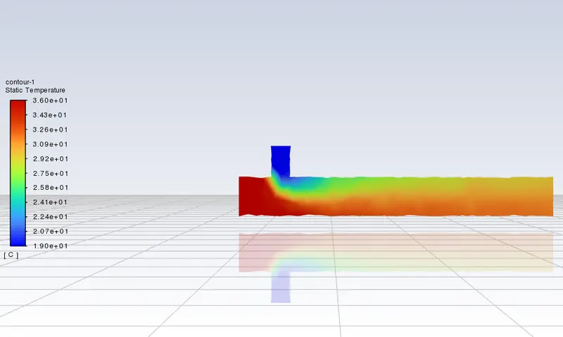
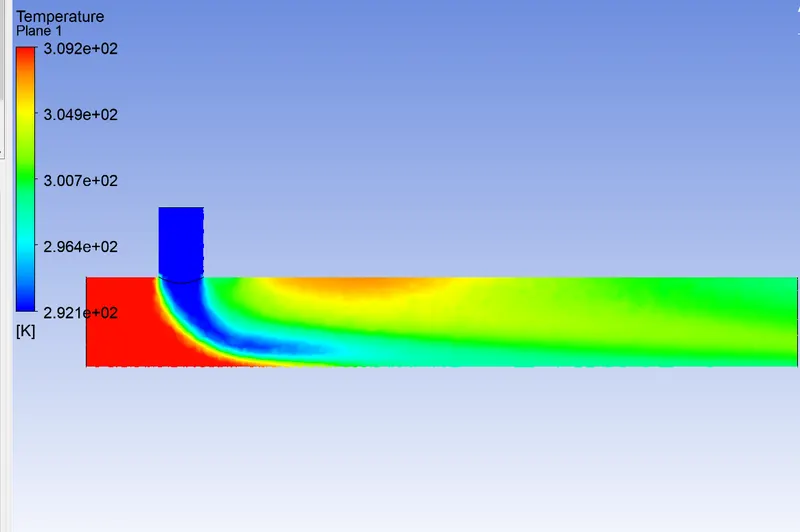
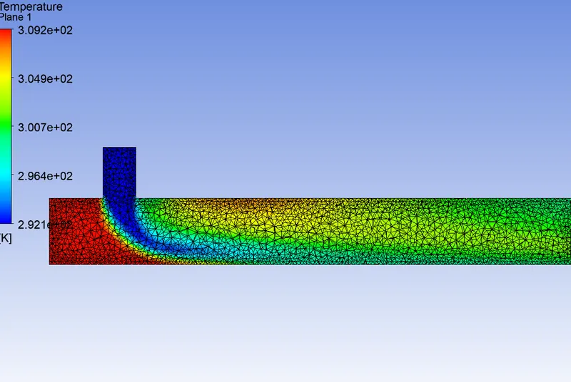
Post-Processing the solution and we get the following rests.
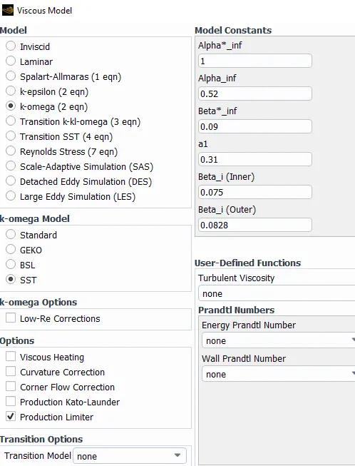
Running for K-Omega SST model
case - 3
Case -4:
No of cases case - 1 case -2 case - 3 case - 4
1. cell counts 26387(1.024e-3) 26387 130956 Tetra Hedral (2e-3m) 130956 Tetra Hedral (2e-3m)
2. Average Outlet Temp (K) 300K 300K 302.7K 302.6K
3. No of Iterations for convergence 80 80 80-140 80-130
Conclusions:
Its mixing effectiveness is different with different momentum ratios and lengths. As we can see the outlet temp is lower for Short tee and the length is a bit higher comparatively. But the effectiveness is much better and efficient in long tee whereas in short, the mixing is not fine.
References: