Modeling of an Electric Vehicle using MATLAB and Simulink
Aim - Create a MATLAB model of an electric car which uses a battery and a DC motor using suitable blocks from the Powertrain block set.
Objectives :
Detailed project report including:
- System-level configuration
- Model parameters
- Results
- Conclusion
Introduction :
Electric Vehicles - There are three main types of electric vehicles (EVs), classed by the degree that electricity is used as their energy source. BEVs, or battery electric vehicles, PHEVs of plug-in hybrid electric vehicles, and HEVs, or hybrid electric vehicles. Only BEVs are capable of charging on a level 3, DC fast charge:
- Level 1 - Level 1 EV charging uses a standard household (120v) outlet to plug into the electric vehicle and takes over 8 hours to charge an EV for approximately 75-80 miles. Level one charging is typically done at home or at your workplace. Level 1 chargers have the capability to charge most EVs on the market.
- Level 2 - Level 2 charging requires a specialized station which provides power at 240v. Level 2 chargers are typically found at workplaces and public charging stations and will take about 4 hours to charge a battery to 75-80 miles of range.
- Level 3 - Level 3 charging, DC fast charging, or simply fast charging is currently the fastest charging solution in the EV market. DC fast chargers are found at dedicated EV charging stations and charge a battery up to 90 miles range in approximately 30 minutes.
The cars which are propelled by one or more traction motors, running on rechargeable batteries are called electric cars. As compared to ICE cars, most of the electric cars provide a higher acceleration mainly due to quickly available high torque from motors and reduced drivetrain frictional losses. A lot of electric cars use a fixed gearbox and have no clutch. Also, a direct motor to wheel configuration can also be used to further reduce the drivetrain friction losses using, a hub motor. Electric vehicles can provide efficiency as high as 70 %.
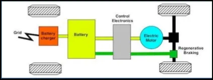
fig: EV Architecture
Powertrain Blockset - Powertrain block set provides a component library for simulating engine subsystems, transmission assemblies, traction motors, battery packs, controller models dynamometers model for virtual testing. It includes fully assembled reference application models of automotive powertrains, including gasoline engine, diesel, hybrid and electric systems.
It provides a standard model architecture that can be reused throughout the development process for design tradeoff analysis, component sizing, control parameter optimization and hardware-in-the-loop testing.
System-Level Configurations and Model Parameters :
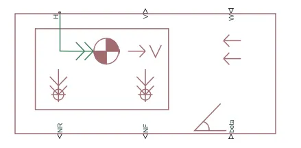
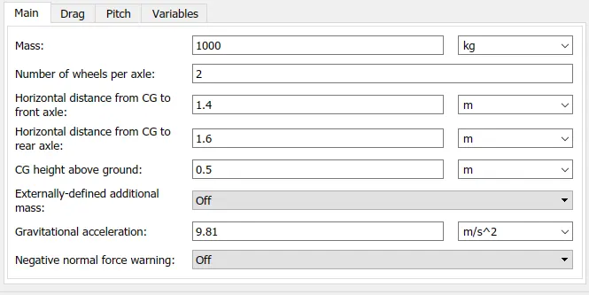
| Vehicle Body | Description | The Vehicle Body block is used in the block diagram of the electric vehicle. It represents a two-axle vehicle body in longitudinal motion and accounts for body mass, aerodynamic drag, road incline and weight distribution between axles. The vehicle can have the same or a different number of wheels on each axle. The vehicle does not move vertically relative to the ground but the suspension dynamics and additional mass can be added optionally. | |||||||||
| Configuration |
|
||||||||||
| Parameters |
The mass of the vehicle is changed to 1000 kg and the rest of the parameters are unchanged. |
||||||||||
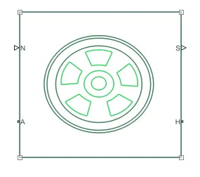
| Tire (Magic Formula) | Description | It represents the longitudinal behaviour of a highway tire characterized by the tire Magic formula. The block is built from Tire-Road Interaction(magic Formula) and Simscape Foundation library Wheel and Axle Blocks. The effects of tire inertia, stiffness and sampling can be included optionally. A set of 4 tires (Magic Formula) blocks is used, 2 for the front axle and 2 for the rear. |
|||||||||
| Configuration |
|
||||||||||
| Parameters |
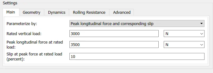
The peak longitudinal force and the corresponding slip parameterization is used with a rated vertical load of 3000 N. |
||||||||||
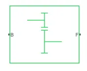
| Simple Gear | Description | It represents a fixed-ratio gearbox and can optionally include gear meshing losses and viscous bearing losses. | |||||||||
| Configuration |
|
||||||||||
| Parameters |
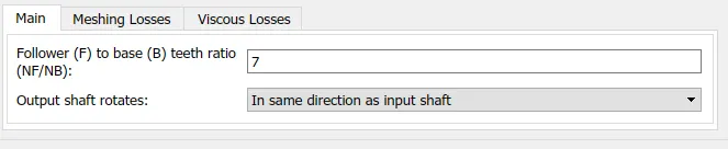
The gear ratio between the base and follower gear is changed to 7 and the output shaft is set to rotate in the same direction as the input shaft. |
||||||||||
| DC Motor | Description | The DC motor block is used to represent the electrical and torque characteristics of a DC motor. This block assumes that no electromagnetic energy is lost.
The motor parameters can either be specified directly or derived from the no-load speed and stall-torque and no information is available on armature inductance, it can be set to some small non-zero value. |
|||||||||
| Configuration |
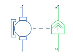
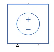
When a positive current flows from the electrical + to - ports, a positive torque acts from the mechanical C to R ports and the motor torque direction can be changed by altering the sign of the back-emf or torque constants. The blue part represents the electric circuit part and the green part represents the mechanical part of the DC motor.
|
||||||||||
| Parameters |
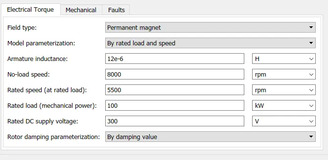
The model parameterization is done by rated load and speed. The rated mechanical power of the motor is 100 kW. The rated speed of the motor is 5500 rpm and the no-load speed is 8000 rpm. Also, the rated DC supply voltage is set to 300 V and the rest of the parameters are unchanged. |
||||||||||
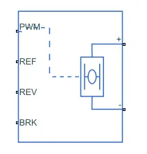
| H-Bridge | Description | This block represents an H-bridge motor drive and can be driven by the Controlled PWM Voltage block in PWM or Averaged mode.
In PWM mode, the motor is powered if the PWM port voltage is above the enabled threshold voltage. In Averaged mode, the ratio of the on-time to the PWM period is defined by the PWM port voltage divided by the PWM signal amplitude. The simulation mode parameter value must be the same for the Controlled PWM Voltage and the H-bridge blocks. If the REV port voltage is greater than the reverse threshold voltage, then the output voltage polarity is reversed. If the BRK port voltage is greater than the Braking threshold voltage, then the output terminals are short-circuited via one bridge arm in series with the parallel combination of a second bridge arm and a freewheeling diode. Voltages at ports PWM, REV and BRK are defined relative to the REF port. |
|||||||||
| Configuration |
|
||||||||||
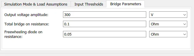
| Parameters | 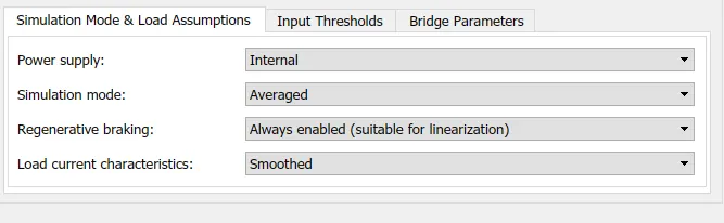 The power supply is set internal and the simulation mode is set to averaged for faster simulation. The regenerative braking is enabled for always.
|
||||||||||
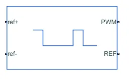
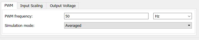
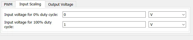
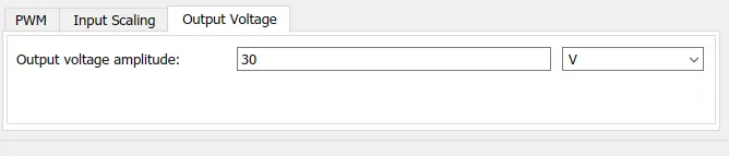
| Controlled PWM Voltage | Description | This block creates a PWM (pulse width modulated) voltage across the PWM and REF ports of the H-bridge. The output voltage is zero when the pulse is low and is equal to the output voltage parameter when high.
The Simulation mode can be set to PWM or Averaged. In PWM mode, the output is a PWM signal. In Averaged mode, the output is constant with a value equal to the averaged PWM signal. |
|||||||||
| Configuration |
|
||||||||||
| Parameters |
|
||||||||||
| Controlled Voltage Source | Description | This block represents an ideal voltage source that is powerful enough to maintain the specified voltage at its output regardless of the current passing through it. The output voltage is V = Vs, where Vs is the numerical value presented at the physical signal port. | |||||||||
| Configuration |
Two of these voltage sources are used, one for the forward command and the other for the braking command. |
||||||||||
| Parameters | The controlled voltage source block does not have any block parameters of its own. It receives input from the longitudinal driver block and gives output to H-bridge block. | ||||||||||
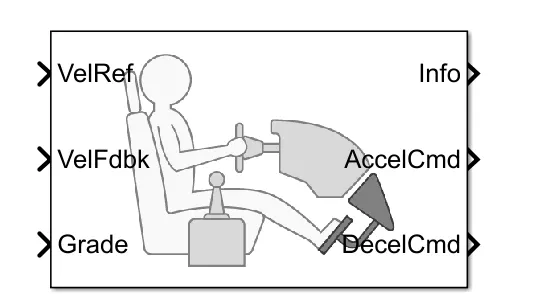
| Longitudinal Driver | Description | It is a parametric longitudinal speed tracking controller for generating normalized acceleration and braking commands based on reference and feedback velocities. This block is simply a modified PI controller. The external input signals can be provided that can disable, override or hold the closed-loop commands determined by the blocks. | |||||||||
| Configuration |
|
||||||||||
| Parameters |
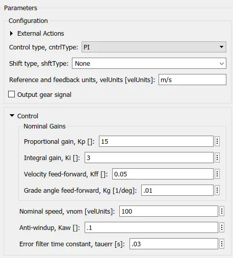
The proportional gain `k_p` is set 15 and the integral gain `k_i` is set 3 for more accurate results. |
Drive Cycle Source - This block generated a standard or user-defined longitudinal drive cycle. The block output is the vehicle longitudinal speed.
The drive cycles can be imported from :
- predefined sources
-
workspace variables, including arrays and time series objects
-
mat, xls, xlsx, or txt files
Final Model :
The Simulink model of the designed electric vehicle can be accessed through this link : EV Model
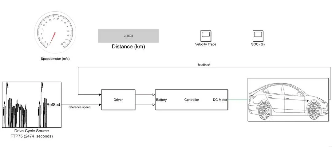
- The Drive Cycle Source provides the reference longitudinal speed to the driver block. There are a number of standard drive cycles to choose such as FTP75, US06, SC03 and many more. The drive cycle can be defined by the user as well through mat, xlsx or text files.
While choosing the required drive cycle in the drive cycle source block, the simulation time needs to be updated because each drive cycle has a different duration. This can either be done manually or simply by clicking the 'Update simulation time' button in the block parameters of the drive cycle source block. - The Driver subsystem block consists of a longitudinal driver block:
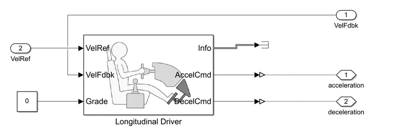
fig: Driver Subsystem
It receives the reference speed signal as input from the drive cycle source and the feedback speed signal from the vehicle body block. The driver block is based on a PI controller and gives the acceleration and deceleration command as output. - Next subsystem consisted of a battery, controller and the DC motor:
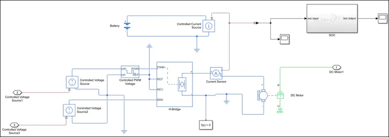
fig: Battery, Controller, DC motor
The subsystem consists of three main blocks: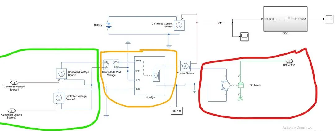
The part highlighted in green is the voltage source. There are two controlled voltage blocks used, one for the acceleration command and the other for the deceleration command and receive their inputs from the longitudinal driver block.
The part highlighted in yellow consists of a controller and an H-bridge. The controller receives the input signal from the controlled voltage sources and generates modulated width pulses as output for the H-bridge. The H-bridge receives the PWM input from the controller along with the brake signal from the second controlled voltage source block.
The part highlighted in red is a DC motor, which receives input from the H-bridge block and in between them is a current sensor. The rotational motion signal is sent as output a mechanical rotational reference is connected.
A battery is attached separately, which is not directly running the DC motor but is used for visualization of the SOC of the battery. The signal from the current sensor goes into the controlled current source block. Thus, the current is generated whenever the vehicle undergoes retardation. This current signal is further processed in a new sub-system SOC which is located at the top right of its sub-system.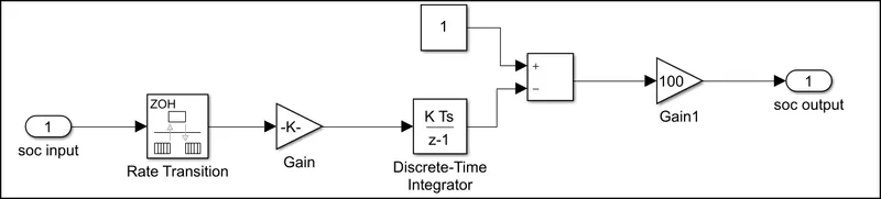
fig: SOC Subsystem
The above substem calculates the SOC fo the battery, getting its input from the current sensor which is added between the H-bridge and the DC motor.
- The third subsystem consists of the Vehicle Body and Tires :
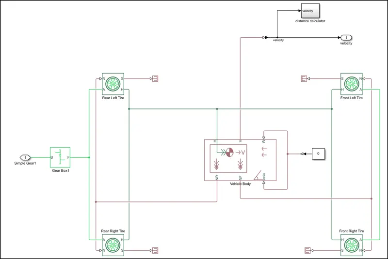
fig: Vehicle Body and Tires
A set of four tire block are used - two for the front axle and two for the rear axle and the required connections are made with the vehicle body block. The normal force signal from the vehicle body block is sent to the normal force input ports of the tires.
The A ports are the mechanical rotational conserving port and receive mechanical rotational input from the gearbox which receives its input from the DC motor.
The H port is the mechanical translational conserving port for the wheel hub and is connected to the H port of the vehicle body.
The output of the vehicle body is Velocity which is sent as feedback to the longitudinal driver block and is separately used to calculate the distance travelled by the vehicle through another subsystem - distance calculator.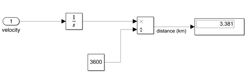
The velocity signal is first integrated to calculate the distance and then divide by 3600 to convert the distance into km.
Results :
The simulations are run for various drive cycles and the results are in the following table.
Simulation Time - It is the time for which the simulation is run. Each drive cycle has its own time duration which needs to be updated in simulation time, each time the drive cycle is changed.
Speed Trace - It is a plot of the reference speed from the drive cycle and the feedback speed from the vehicle body.
SOC (%) - It is the state of charge of the battery which decreases when the vehicle accelerated and slightly increases when the vehicle decelerates.
Distance Travelled - It is the total distance travelled by the vehicle following a particular drive cycle and its duration.
| Drive Cycle | Results | |
| FTP 75 | Simulation Time | 2474 seconds |
| Speed Trace | 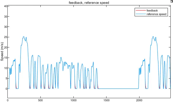 |
|
| SOC (%) | 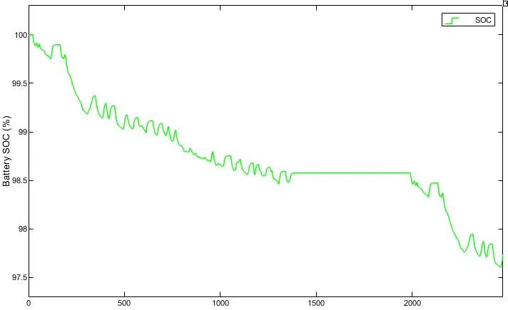 |
|
| Distance Travelled | 5.0003 km | |
| US06 | Simulation Time | 600 seconds |
| Speed Trace | 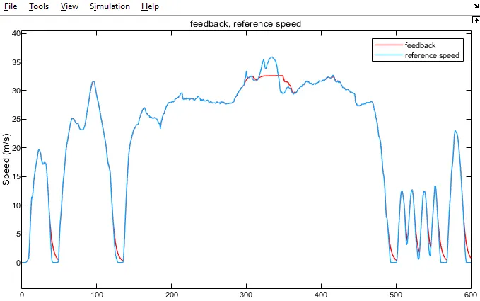 |
|
| SOC (%) | 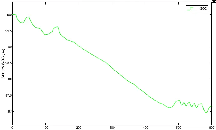 |
|
| Distance Travelled | 3.5994 | |
| SC03 | Simulation Time | 600 |
| Speed Trace | 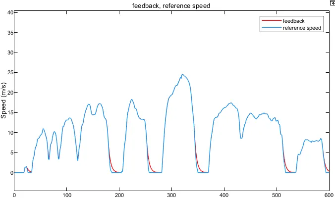 |
|
| SOC (%) | 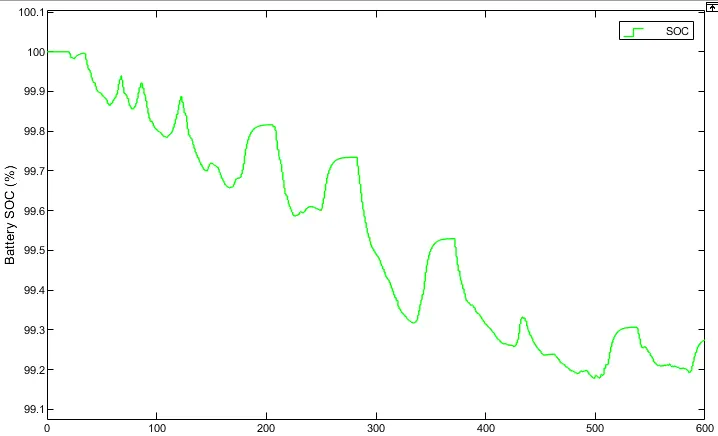 |
|
| Distance Travelled | 1.6218 km | |
| HWFET | Simulation Time | 765 seconds |
| Speed Trace | 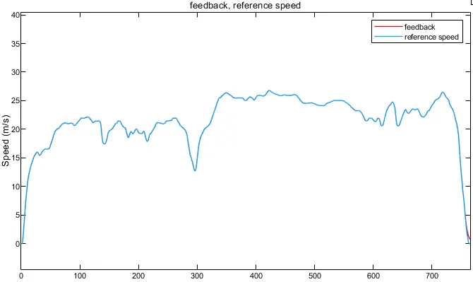 |
|
| SOC (%) | 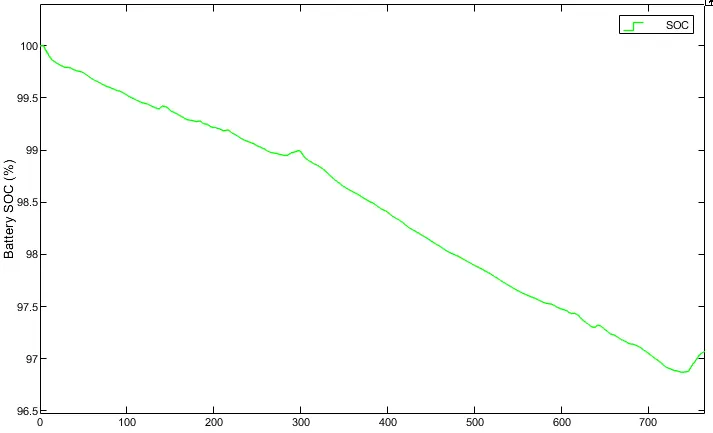 |
|
| Distance Travelled | 4.5866 km | |
| NYCC | Simulation Time | 5988 seconds |
| Speed Trace | 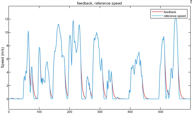 |
|
| SOC (%) | 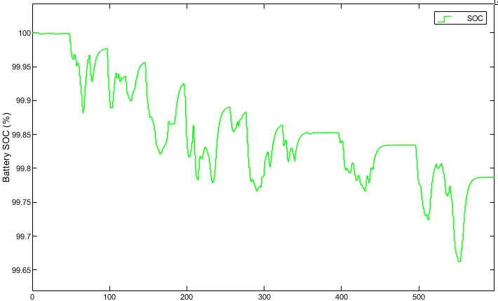 |
|
| Distance Travelled | 0.5546 km | |
| LA92 | Simulation Time | 1435 seconds |
| Speed Trace | 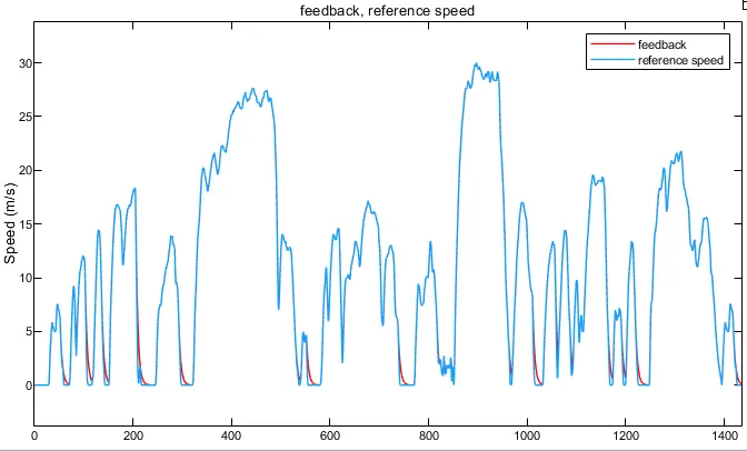 |
|
| SOC (%) | 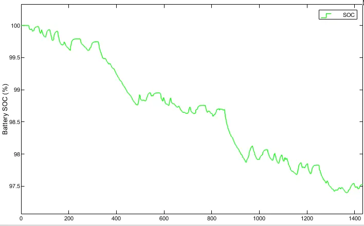 |
|
| Distance Travelled | 4.4418 km | |
Conclusion :
- In the speed trace plots for all the drive cycles which are observed in this study, the feedback speed plot and the reference speed plot overlap each other almost completely but there are regions where both the speeds are different. It is when the vehicle is decelerating.
The reference speed plot falls sharply but the feedback speed does not. This is due to the inertia of the vehicle body. As the inertia of the vehicle body is higher, it takes a longer duration for it to decelerate.
That is why the overlapping is not 100%. - Also, in the case of the US06 drive cycle, the reference speed plot is much higher than the feedback speed plot at a duration of 300 seconds. Here, the reference speed goes as high as 35 m/s while the maximum feedback speed is limited to around 32.5 m/s. This is because of the powertrain i.e. either the motor is not powerful enough, the battery voltage is less, the vehicle body is too heavy, etc.
- The battery's state of charge for each drive cycle can be visualized from the SOC plot. As long as the vehicle is accelerating the SOC is decreasing but as soon as the deceleration starts, the SOC plot goes slightly up. This is because the battery is being charged, due to regenerative braking during deceleration.
References :