Effects of Reynolds number on Flow over a Cylinder

Objective

To study the flow over a cylinder by changing the Reynolds number (Re) and observing the changes in pressure and velocity. In this study, the following steps are performed:

1. A baseline case is run and the resulting Reynolds number is computed
2. Three more cases are studied where the Reynolds number is increased by 20%, 40% and 100% of the original Re number. The resulting inlet velocities are then computed.
3. Velocity and Pressure contour plots and animations are then obtained, which is followed by a discussion of the results.

Introduction

Computational Fluid Dynamics (CFD) is the process of mathematically modeling a physical phenomenon involving fluid flow and solving it numerically with the help of computing and processing power of a computer. In a CFD software analysis, the examination of fluid flow in accordance with its various physical properties such as velocity, pressure, temperature, density and viscosity are conducted. These properties need to be reviewed simultaneously in order to generate an accurate solution. A mathematical model of the physical case and a numerical method are used in a CFD software tool to analyze the fluid flow. The central mathematical description for all theoretical fluid dynamics models is given by the Navier-Stokes equations, which describe the motion of viscous fluid domains with three major equations, which are the conservation of mass, momentum and energy, respectively [1].

Theory

In this project, a few major parameters relevant to the project will be discussed in further detail

1. Reynolds number: The Reynolds number is the ratio of inertial forces to viscous forces within a fluid which is subjected to relative internal movement due to different fluid velocities [2]. It is defined by the formula:

where:

• ρ is the density of the fluid (SI units: kg/m3)
• u is the flow speed (m/s)
• L is a characteristic linear dimension (m)
• μ is the dynamic viscosity of the fluid (Pa·s or N·s/m2 or kg/(m·s))
• ν is the kinematic viscosity of the fluid (m2/s).

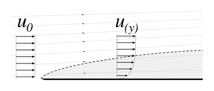
2. Boundary layer: It is the thin layer of fluid in the immediate vicinity of a bounding surface formed by the fluid flowing along the surface [3]. The fluid's interaction with the wall induces a no-slip boundary condition (zero velocity at the wall), which increases slowly above the surface until it returns to the bulk flow velocity. The thin layer consisting of fluid whose velocity has not yet returned to the bulk flow velocity is called the velocity boundary layer.

Project Setup

For the baseline case, air will be used as the working fluid with a velocity of 10 m/s. A cylinder of diameter 0.04m with a length of 0.05 m will be used.

The ambient air temperature is 293 K. At this temperature, the kinematic viscosity of air is 1.516 x 10^-5 m²/s. Using these values, the Reynolds number Re = 26,385

For the remaining cases, the Reynolds number is now increased by 20%, 40% and 100%. Using these Reynolds number values, the inlet velocity values are recalculated:

Case No	Reynolds number	Inlet Velocity (m/s)
1	26,385	10
2	31,662	12
3	36,939	14
4	52,770	20

The next step is to calculate the simulation times. Case 1 will be used as a sample calculation. Here, we assume a computational domain length of 1 m.

With a velocity of 10 m/s, it would take 0.1 s for the flow to reach the outlet, also called the ‘flow through time’ (time=distance/velocity). For the simulation, we then double the value of this time. We break this simulation time down into 20 intervals, which is the step time for a very smooth transition during the animation sequence.

Case No	Computational Domain Length (m)	Inlet Velocity (m/s)	Flow through time (s)	Simulation time (s)	Step time (s)
1	1	10	0.1	0.2	0.01
2	1	12	0.08	0.16	0.008
3	1	14	0.07	0.14	0.007
4	1	20	0.05	0.1	0.005

3D model

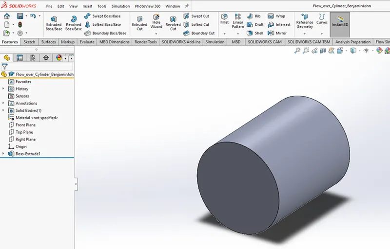
The first stage is to set up the model so that we can run the simulations. In this experiment, we will use a pipe of diameter 0.04 m. First, create a sketch on the front plane container a circle of diameter 0.04m. Extrude it to a length of 0.05 m. We are now ready to set up the simulation model.

Simulation setup

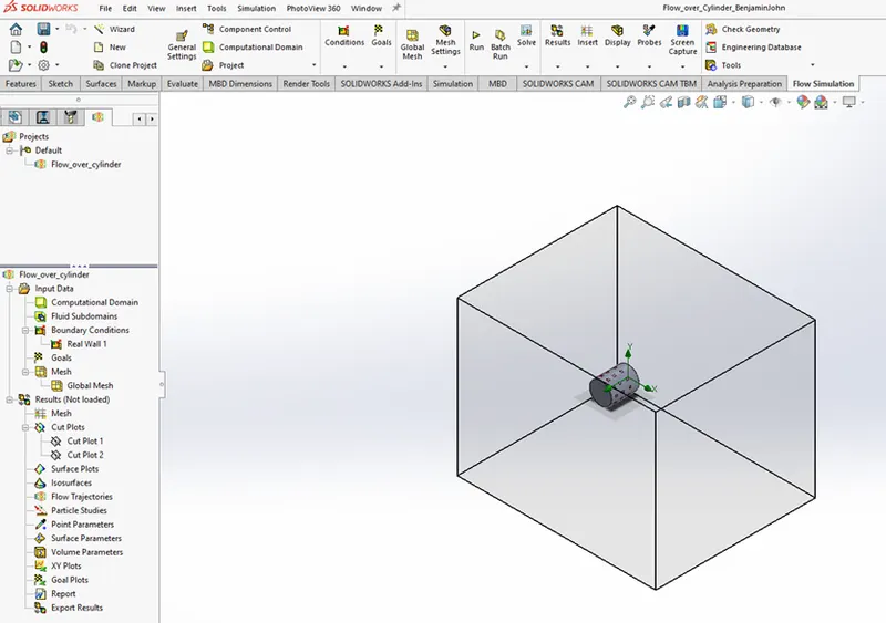
1. New Project: Create a new project by clicking on ‘Wizard’ in the flow simulation tab and provide a project file name. Set up the following:

• Analysis type: External (as the flow is measured outside the object)
• Select the Time Dependent option in the Physical Features option. Add the simulation time and step time for each case.
• Working Fluid: Air
• Flow Type: Laminar and Turbulent
• Add the inlet velocity in the X direction for each case.
• Leave the wall as adiabatic and don’t add any roughness to the pipe.

This will now create a bounding box outside the cylinder.

2. Boundary conditions: Set the wall of the cylinder to be a ‘Real wall’.
3. Mesh: Edit mesh settings to level 5. Select the ‘Advanced channel refinement’ option as this will make the velocity profiles more accurate.
4. Plots: In order to visualize the results, plots need to be set up. Add cut plots at the middle of the cylinder length for velocity and pressure.

Now, the simulation can be run, and then save the resulting plots and animation sequences for each case.

Results & Discussion

A detailed discussion is provided below (right after all the plots). In each case, the velocity and pressure plots are added, which is followed by an animation sequence for each one as it is time dependent.

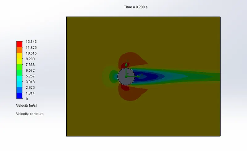
Case 1: Velocity plot, Inlet velocity = 10 m/s, Simulation time = 0.2 s

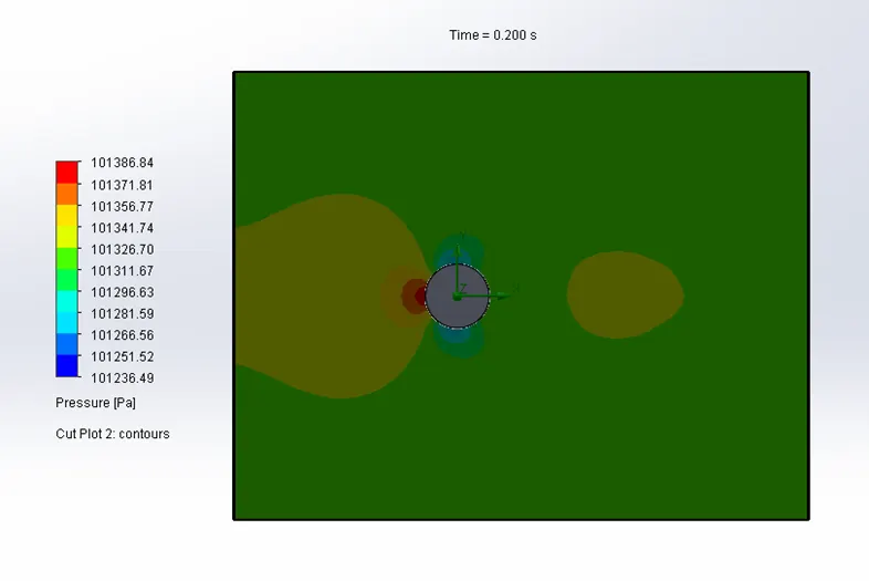
Case 1: Pressure plot, Inlet velocity = 10 m/s, Simulation time = 0.2 s

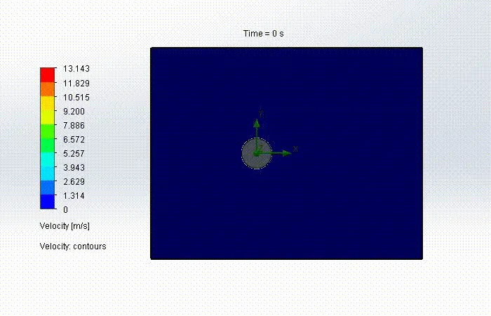
Case 1: Velocity animation, Inlet velocity = 10 m/s, Simulation time = 0.2 s

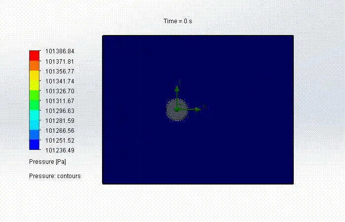
Case 1: Pressure animation, Inlet velocity = 10 m/s, Simulation time = 0.2 s

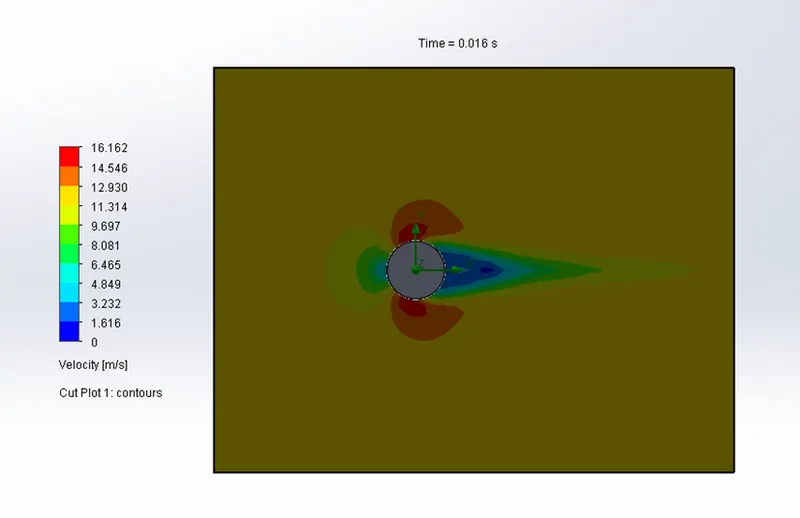
Case 2: Velocity plot, Inlet velocity = 12 m/s, Simulation time = 0.16 s

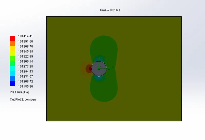
Case 2: Pressure plot, Inlet velocity = 12 m/s, Simulation time = 0.16 s

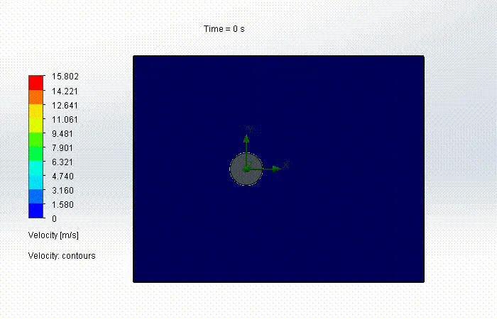
Case 2: Velocity animation, Inlet velocity = 12 m/s, Simulation time = 0.16 s

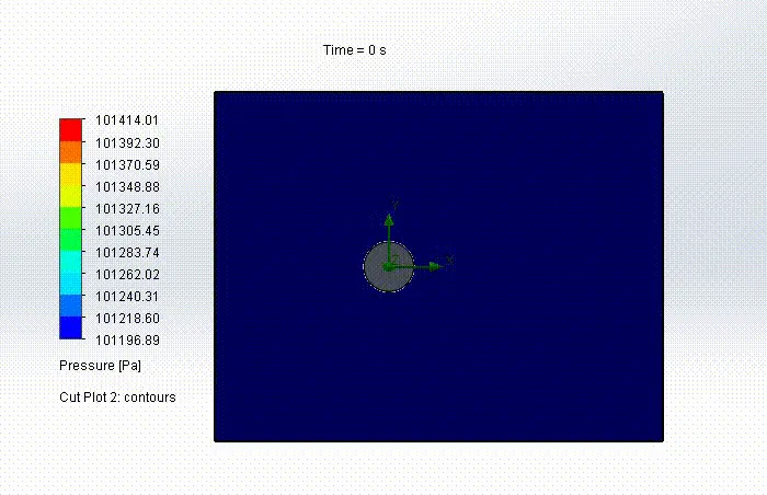
Case 2: Pressure animation, Inlet velocity = 12 m/s, Simulation time = 0.16 s

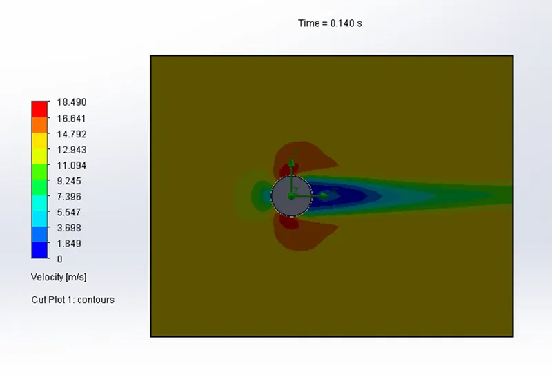
Case 3: Velocity plot, Inlet velocity = 14 m/s, Simulation time = 0.14 s

Case 3: Pressure plot, Inlet velocity = 14 m/s, Simulation time = 0.14 s

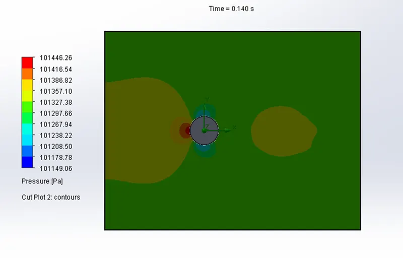
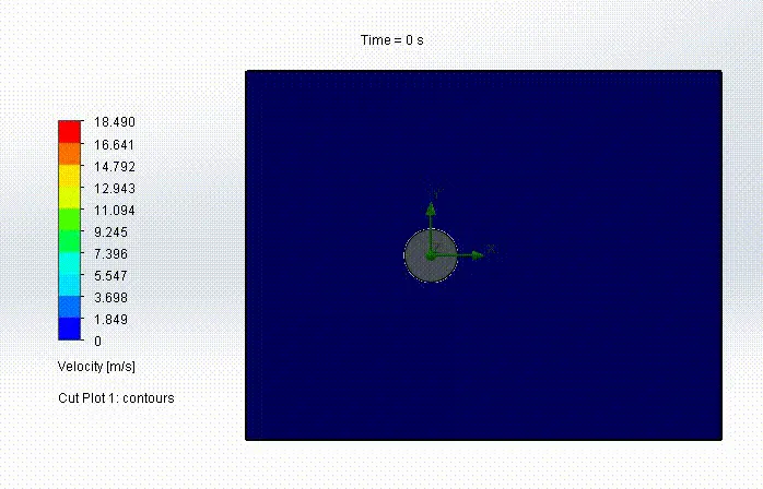
Case 3: Velocity animation, Inlet velocity = 14 m/s, Simulation time = 0.14 s

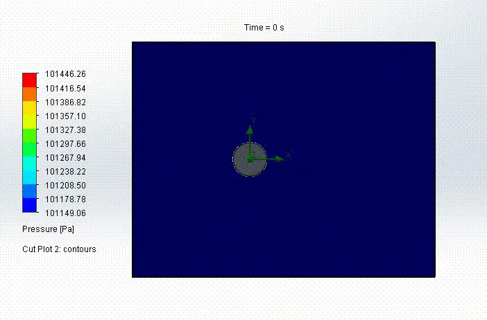
Case 3: Pressure animation, Inlet velocity = 14 m/s, Simulation time = 0.14 s

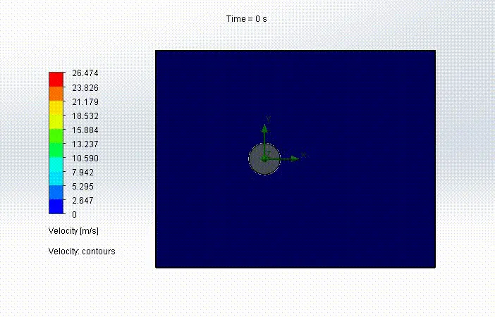
Case 4: Velocity plot, Inlet velocity = 20 m/s, Simulation time = 0.10 s

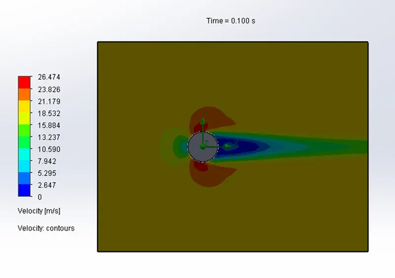
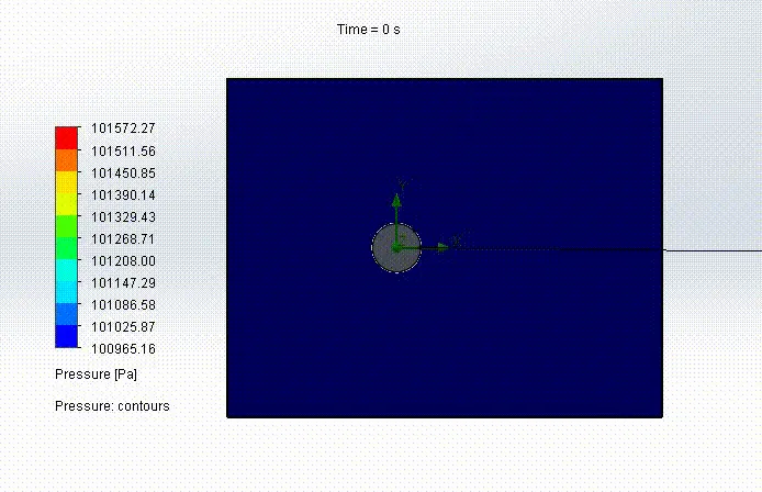
Case 4: Pressure plot, Inlet velocity = 20 m/s, Simulation time = 0.10 s

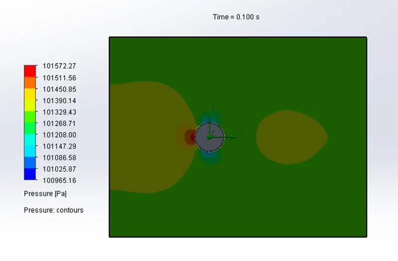
Case 4: Velocity animation, Inlet velocity = 20 m/s, Simulation time = 0.10 s

Case 4: Pressure animation, Inlet velocity = 20 m/s, Simulation time = 0.10 s

The following observations can be noted:

1. Doubling the flow through time to obtain the simulation time appears to make the flow approach a more continuous variation in the velocity and pressure profiles. This is evident from the animation sequences displayed at all Reynolds numbers.
2. In the flow, the maximum velocity appears on the top ends of the cylinder, while the minimum velocities appear right behind the cylinder. On the other hand, the maximum pressure appears right in front of the cylinder, along the midpoint. The minimum pressure appears on top of the cylinder, along the same region as the maximum velocity. This point is also known as the stagnation point.

3. Increasing the Reynolds number increases the maximum velocity and pressure experience on the cylinder. This is expected as the inlet velocity and Reynolds number are directly proportional to each other, as seen in the Reynolds number formula.
4. At low Reynolds numbers, we can model the flow as a potential flow, when using an inviscid and incompressible fluid. This would be using ideal conditions.
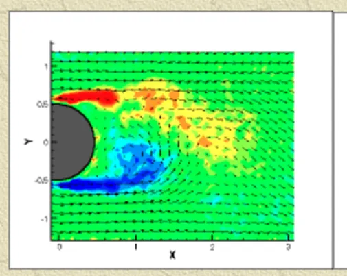
5. At high Reynolds numbers (usually > 400,000), the flow properties change to the point where the flow becomes turbulent. In this case, vortex shedding occurs behind the cylinder in alternating patterns, as shown below [4]. This can be done as a future study.

Sources

[1] https://www.simscale.com/docs/simwiki/cfd-computational-fluid-dynamics/what-is-cfd-computational-fluid-dynamics/

[2] Wikipedia contributors. (2022, February 23). Reynolds number. In Wikipedia, The Free Encyclopedia. Retrieved 01:47, April 13, 2022, from https://en.wikipedia.org/w/index.php?title=Reynolds_number&oldid=1073588192

[3] Wikipedia contributors. (2022, March 29). Boundary layer. In Wikipedia, The Free Encyclopedia. Retrieved 01:54, April 13, 2022, from https://en.wikipedia.org/w/index.php?title=Boundary_layer&oldid=1080021986

[4] https://eng-web1.eng.famu.fsu.edu/~shih/succeed/cylinder/cylinder.htm#Wake