Implicit vs Explicit FEA: Differences, Time Step and When to Use Each

In short

• Implicit FEA solves for equilibrium at the end of each increment using the stiffness matrix and Newton iterations. Increments can be large; each one is expensive.
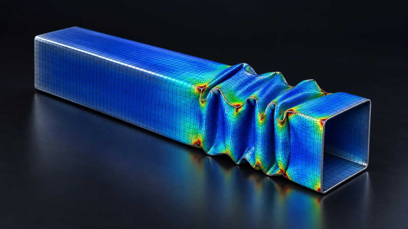
• Explicit FEA marches forward in very small time steps using only what is already known. No stiffness matrix, no iterations, but the step must stay below a stability limit, about one microsecond for typical steel crash meshes.
• Use implicit for static, slow and vibration problems. Use explicit for short, violent events such as crash, drop and impact, and for problems with severe contact that implicit struggles to converge.
• Both methods handle non-linearity and contact. The choice is about time scale and cost, not about which one is "more accurate".

The one-line difference

Every structural FE solver works with the same equation of motion, written for the whole mesh:

M·ü + C·u̇ + Fint(u) = Fext(t)

where M is the mass matrix, C damping, Fint the internal forces from element stresses (which equal K·u for a linear problem) and Fext the applied loads. The two methods differ only in how they step this equation from time t to t + Δt:

• Implicit: the state at t + Δt appears on both sides of the equation, so the solver has to solve a system of equations (usually non-linear) to find it.
• Explicit: the state at t + Δt is calculated directly from the state at t, which is already known. No system of equations is solved.

How implicit FEA works

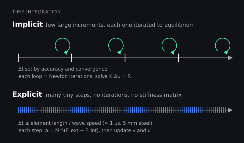
In an implicit analysis the solver guesses the displacement at the end of an increment, computes the internal forces, and compares them with the external loads. The difference is the residual. It then uses the tangent stiffness matrix to correct the guess (KT·Δu = R) and repeats until the residual and the displacement correction are below tolerance. This is the Newton-Raphson method, and each repetition is one equilibrium iteration.

A static analysis is simply the case with no inertia: there is no real time, only load increments. For dynamic problems, implicit codes use integration schemes such as Newmark or HHT (Hilber-Hughes-Taylor), which are unconditionally stable for linear problems. That means the time increment is chosen for accuracy and convergence, not stability, and can be thousands of times larger than an explicit step.

The price is paid in each increment. Assembling and factorising a large stiffness matrix needs a lot of memory and CPU, and the cost grows faster than linearly with model size. If the model changes state abruptly (contact opening and closing across many surfaces, buckling, material failure), Newton iterations can fail to converge, and the solver cuts back the increment, sometimes until it gives up.

How explicit FEA works

Explicit solvers usually use the central difference method with a lumped (diagonal) mass matrix. Each time step is the same short recipe:

1. Compute the internal forces from the current element stresses and the contact forces.
2. Get accelerations directly: a = M⁻¹·(Fext − Fint). Because M is diagonal, this is a division per degree of freedom, not a matrix solve.
3. Update velocities and displacements, then the element strains and stresses, and move to the next step.

Each step is cheap and the work splits easily across many CPU cores, which is why full-vehicle crash models with millions of elements are practical. The catch is stability. Central difference is only conditionally stable: the time step must be smaller than the time a stress wave takes to cross the smallest element. In simple terms:

Δtcrit ≈ Lmin / c, with wave speed c ≈ √(E/ρ)

Shells and solids use slightly different expressions, and solvers multiply the result by a safety factor (LS-DYNA's default time step scale factor is 0.9), but the idea is the same: smaller or stiffer or lighter elements mean a smaller time step.

Worked example: how many steps does a crash run need?

Take a body-in-white crash model meshed mostly with 5 mm steel shells (E = 210 GPa, ρ = 7,850 kg/m³).

1. Wave speed: c = √(210 × 10⁹ / 7,850) ≈ 5,170 m/s.
2. Critical step for a 5 mm element: 0.005 / 5,170 ≈ 0.97 µs. With a 0.9 scale factor, Δt ≈ 0.87 µs.
3. A frontal crash event lasts about 100 ms, so the run needs 0.1 / (0.87 × 10⁻⁶) ≈ 115,000 time steps.

Now suppose a few badly sized 1 mm elements slip into the mesh around a weld flange. The whole model must run at their time step: 0.9 × 0.001 / 5,170 ≈ 0.17 µs, or about 575,000 steps. One small patch of mesh has made the run five times slower. Aluminium gives almost the same wave speed (about 5,090 m/s), so the same logic applies to aluminium structures.

This is why crash meshing guidelines specify a minimum element size, and why explicit users check the time step history before submitting a job. When a few small elements cannot be avoided, the common fix is mass scaling: adding non-physical mass to just those elements so their time step rises. Because Δt is proportional to √ρ, getting those 1 mm elements back to 0.87 µs needs their density raised about (0.87 / 0.17)² ≈ 25 times. That is acceptable for a handful of elements away from the load path, but not for a whole component. Solvers report the added mass (in LS-DYNA it is controlled from *CONTROL_TIMESTEP), and teams usually keep it to a small fraction of total model mass and check that it is not in the region that matters.

Implicit vs explicit FEA at a glance

	Implicit	Explicit
What is solved each increment	System of equations with the stiffness matrix, iterated to equilibrium	Direct update from known values, no stiffness matrix
Stability	Unconditionally stable for linear dynamics (Newmark, HHT)	Conditionally stable: Δt below the critical step
Typical time increment	Large (set by accuracy and convergence)	Very small, often around a microsecond
Cost per increment	High; memory hungry; grows faster than model size	Low; scales roughly with element count
Best suited event duration	Static, seconds to hours, low-frequency dynamics	Milliseconds: impacts, crashes, blasts
Contact	Supported; convergence gets hard with many changing contacts	Robust with large, changing contact
Main risk	Non-convergence	Silent errors from bad energy balance or too much mass scaling
Key checks	Convergence history, residuals, reaction forces	Energy balance, hourglass energy, added mass, time step history

When to use implicit FEA

• Linear and non-linear static stress analysis: brackets, chassis parts, pressure vessels, bolted joints with preload.
• Modal (natural frequency) analysis, harmonic and random vibration, and the stiffness work that feeds NVH.
• Linear buckling, and post-buckling with arc-length (Riks) methods.
• Thermal and thermal-stress analysis, creep and other slow processes.
• Durability and fatigue load cases, which are usually built from static or modal results.
• Springback after sheet metal forming.

When to use explicit FEA

• Vehicle crash and occupant safety: frontal, side, pole and pedestrian impacts.
• Drop tests of phones, laptops and packaging, and bird strike or projectile impact.
• Blast and high-velocity events.
• Sheet metal forming, forging and other large-deformation manufacturing processes.
• Quasi-static problems with severe contact or instability that implicit cannot converge, such as rubber seals, snap-fits or crushing. Here the load is applied slowly enough that inertia stays small, and you check that kinetic energy remains a small fraction of internal energy (a common rule of thumb is under about 5 to 10%).

Common myths about implicit and explicit FEA

• "Implicit cannot handle contact." It can, and does every day in bolted joints and assemblies. What is hard is convergence when many contacts change state at once.
• "Explicit is more accurate." Neither is inherently more accurate. Each is accurate for the problems it suits. An explicit run of a slow static problem can be badly wrong if inertia effects creep in.
• "Explicit is only for dynamics." Many quasi-static problems run in explicit, with careful loading rates and energy checks.
• "You must choose one." Many workflows chain them: forming in explicit, springback in implicit; or an implicit preload (gravity, bolt tension) followed by an explicit impact.

How to check your results

Implicit checklist

• The analysis converged at every increment, with no excessive cutbacks.
• Reaction forces balance the applied loads.
• Deformed shape and stress hot spots make physical sense; peak stresses at singularities (sharp corners, point loads) are read with care.
• For non-linear runs, the load-displacement curve is smooth where you expect it to be.

Explicit checklist

• Total energy stays roughly constant; external work is accounted for by internal, kinetic and contact energy.
• Hourglass energy stays small relative to internal energy (10% is a widely used upper limit).
• Added mass from mass scaling is small and away from the critical load path.
• The time step history has no sudden drops caused by distorted elements.

Which solvers use which method?

Most major codes offer both, under different names: Abaqus/Standard (implicit) and Abaqus/Explicit; Ansys Mechanical (implicit) and Ansys LS-DYNA (explicit-first, with an implicit solver too); Altair OptiStruct (implicit) and Altair Radioss (explicit). LS-DYNA is best known for explicit crash work but contains a full implicit solver. Knowing which method sits behind a menu is more useful than memorising product names.

Where to learn this properly

If you are moving into CAE, start with the theory and a few small models in each method, then specialise. Useful next steps on Skill-Lync:

• Basics of FEA: Explicit and Implicit FEA, for the fundamentals with hands-on models.
• LS-DYNA for Structural Mechanics/FEA, for explicit dynamics, contact and material models.
• Crashworthiness Analysis using HyperMesh and Radioss, for full crash load cases.
• Post Graduate Program in CAE, which combines meshing, implicit and explicit analysis in industry projects.

Frequently asked questions

Is LS-DYNA implicit or explicit?

Both. It is best known for explicit analysis such as crash and impact, but it also has an implicit solver for static, modal and slow dynamic problems, and can switch between them in one run.

Why is the explicit time step so small?

Because the central difference scheme is only stable if information (a stress wave) does not cross more than one element per step. In steel that wave travels at about 5,000 m/s, so millimetre-sized elements give microsecond steps.

Can I run a static analysis in an explicit solver?

Yes, as a quasi-static analysis, by applying the load slowly and confirming that kinetic energy stays small compared with internal energy. It is useful when implicit fails to converge, but implicit is usually faster and cleaner for genuinely static, smooth problems.

What is mass scaling, and is it cheating?

It adds artificial mass to small elements so the explicit time step can be larger. Used sparingly and reported, it is standard practice. Used heavily, it changes the dynamics and the answer.

Do "implicit" and "explicit" mean the same thing in CFD?

The mathematical idea is the same (whether the new state appears on both sides of the update), but in CFD the terms usually describe how the flow equations are integrated in time, which ties to the CFL number rather than to structural wave speed.

Which should a fresher learn first?

Implicit linear static analysis first, because it builds intuition about boundary conditions, meshes and stresses. Then move to non-linear implicit and explicit dynamics, which is where most automotive crash and safety jobs sit.

Sources and further reading

• LS-DYNA Support, Mass scaling (TSSFAC, DT2MS and added mass)
• Ansys LS-DYNA, Technical Guide for Explicit Analyses
• Wikipedia, Explicit and implicit methods (mathematical background)