Wide Open Throttle Condition for GM EV1 Car

Hill Climbing Power:

Aim: To find the Hill-Climbing power of TATA Ultra Truck.

Objective: To find the ratio of hill-climbing power required by fully loaded Tata ultra truck to the half-loaded one.

Specification:

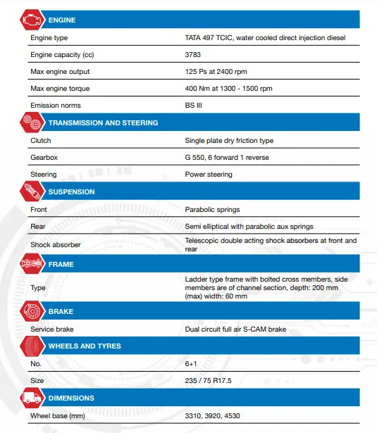
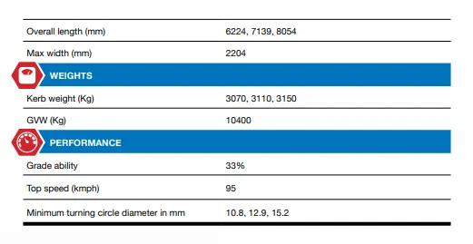
Name of the Truck: TATA Ultra 1012

Calculation:

For Full-load Condition:

Kerb Weight = 3150 kg

GVW = 10400 kg

Payload = GVW – Kerb weight

Payload = 10400-3150 = 7250 kg

Gradeability = 33%

Grade angle = 18.26 degree

Speed(V) = 50kmph = 13.9m/s

Hill Climbing Force,

Fhc = m*g*sinα

Fhc = 10400*9.81* sin(18.26) = 570N

Phc =Fhc * V = 570*13.99 = 7.9KW

For Half-load Condition:

Kerb Weight = 3150 kg

GVW = 10400 kg

Payload = GVW – Kerb weight

Payload = 10400-3150 = 7250 /2 = 3625 kg

Gradeability = 33%

Grade angle = 18.26 degree

Speed(V) = 50kmph = 13.9m/s

Hill Climbing Force,

Fhc = m*g*sinα

Fhc = 6775*9.81* sin(18.26) = 371N

Phc =Fhc * V = 371*13.99 = 5.2KW

Ratio of Hill climbing power = Phc(Full-load)/ Phc(half-load)

= 7.9/5.2 = 1.5

Result:

1. The hill-climbing power required by fully loaded Tata ultra truck is 7.9KW.
2. The hill-climbing power required by half loaded Tata ultra truck is 5.2KW.
3. The ratio of hill-climbing power required by fully loaded Tata ultra truck to half-loaded one is 1.5

Conclusion:

As the Load on the truck increases, more hill climbing power will be required.

Length of Flyover:

Aim: To plan a flyover that is to be constructed on a National highway.

Objective: To calculate the minimum length of the flyover, considering the minimum height at the summit to be 5.5 meters considering Gradeablity for trucks.

Introduction:

Gradeability by definition is the ability of a commercial vehicle to negotiate a grade(slope/acclivity) in Gross Vehicle Weight (GVW) condition and it can vary from 0% to 45% (maximum). A 45° gradient is equivalent to 100%. In other words, gradeability is the highest grade a vehicle can ascend maintaining a particular speed.

Calculation:

Height of the flyover(h) = 5.5m

Gradeability = 33%

Grade angle(ψ">ψ) = 18.26degree

sinψ">ψ = height of the flyover/ Length of the flyover

Length of the flyover(L) = 5.5/sin(18.26) = 17.6m

Results:

1. The Minimum Length of the flyover is 17.6m

Driver-glider Model:

Aim: To Prepare a new drive cycle excel file and revise the Driver-glider model.

Objective: To open the driver-glider library and revise the model according to our drive cycle.

Model:

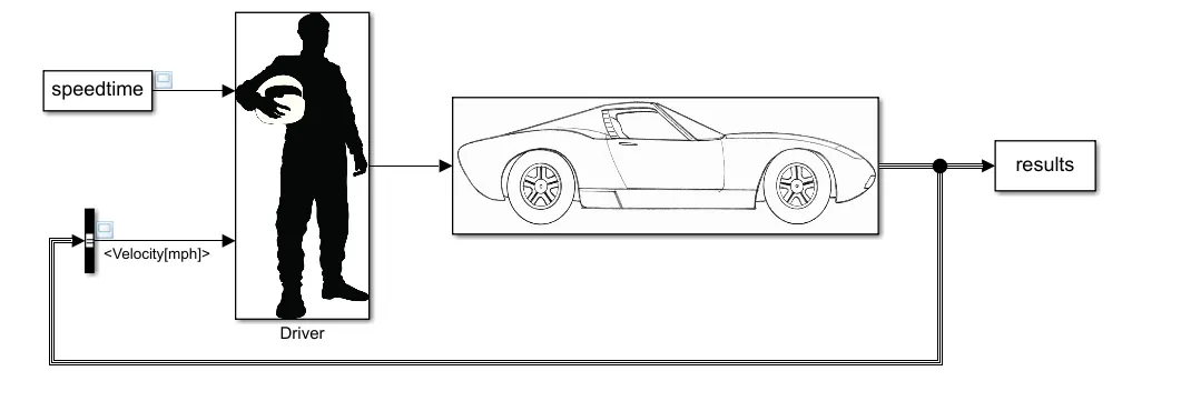
Revising the drive cycle,

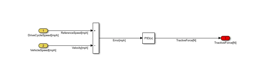
Driver Block-PID:

Glider Block:

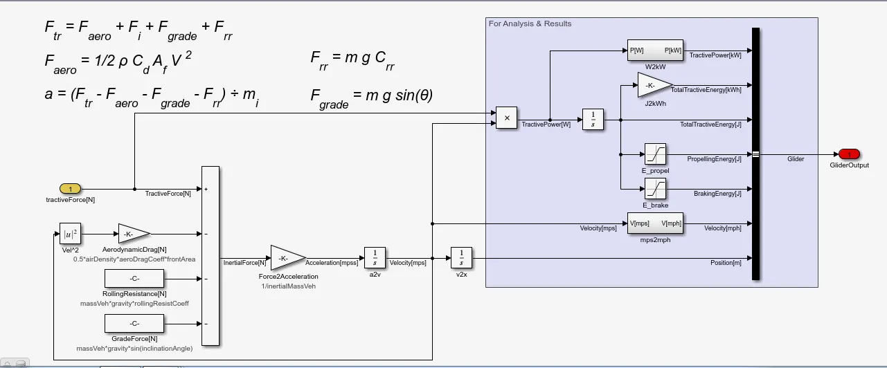
Link to the model: https://drive.google.com/file/d/1BO6cP3O6RLxT6t-pVME8r-ggsYPBpdIp/view?usp=sharing

Link to the Excel sheet: https://drive.google.com/file/d/1mccWcBbbz140NHCg45C-W1WVO76vjOM4/view?usp=sharing

Explanation:

Initially the driver glider library is unlocked and the model of the driver glider is opened.

The default block of the model is removed and a 'from workspace' block is added to create our drive cycle.

An excel file(speedtime) is imported to MATLAB to give inputs to the from workspace block(drive cycle).

Once the drive cycle is ready we can enter the glider block and edit the inclination angle under the grade force block. In this case, inclination angle is set to 5degrees.

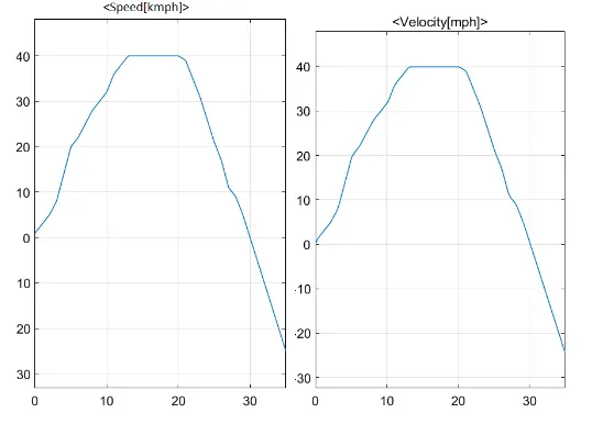
The scopes of velocity in mph and kmph are interconnected.

The driver_glider model is made to run.

Results:

The driver_glider model is made to run for 35 seconds as the drive cycle is of 30 seconds and the following plots are obtained,

WOT of GM EV1 Car:

Aim: To model the WOT (Wide Open Throttle) response of GM EV1 car.

Objective: To calculate the performance characteristics of the real car and compare it with 5% change in the parameters of the same vehicle.

Introduction:

The General Motors EV1 was an electric car produced and leased by General Motors from 1996 to 1999. It was the first mass-produced and purpose-designed Electric vehicle of the modern era from a major automaker and the first GM car designed to be an electric vehicle from the outset.

Calculations and Program code:

Considering original parameters:

Drag coefficient(Cd) = 0.19

Rolling resistance coefficient(µrr) = 0.0048

Frontal area(A) = 0.18m^2

Efficiency of coupling(ηg) = 95%

Kerb weight = 1400kg

Payload = 140kg

GWV = 1540kg

Gear ratio(G) = 11

Radius of wheel = 0.3m

Critical Speed = 19.8m/s

Max. Torque = 140Nm

Angular speed of motor = 733rad/s

Power = 102KW( above critical speed)

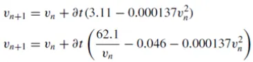
The max torque is constant until the motor reaches critical speed,

%Program to calculate the performance characteristics of a car
clear all
close all
clc

t = linspace(0,40,401); %Time array for drivecycle
v = zeros(1,401);       %Velocity array
dt = 0.1;               %increase in time by 0.1sec

%Loop for above and below critical speed
for i=1:400
    %Below citical speed(19.8m/s)
    if v(i)<=19.8;
        v(i+1) = v(i) + dt*(3.11 - 0.000137*(v(i)^2));
    %Above critical speed
    elseif v(i)>19.8;
        v(i+1) = v(i) + dt*((62.1/v(i)) - 0.046 - (0.000137*(v(i)^2)));
    %If speed of vehicle is above top speed
    elseif v(i)>=35.7
        v(i+1)= v(i);

    end
end

%coverting speed into Kmph
v = v.*(3.6);

%Plotting the figure
figure(1)

plot(t,v);
xlabel('Time (seconds)');
ylabel('Velocity (kmph)');


%End of program

Increasing the parameters of vehicle by 5%:

Drag coefficient(Cd) = 0.19

Rolling resistance coefficient(µrr) = 0.0048+0.00024 = 0.005

Frontal area(A) = 0.9 m^2

GWV = 1638kg

Radius of wheel = 0.315m

Since there is 5% change in the parameters, there is a change in the equation.

%Program to calculate the performance characteristics of a car(5% change)
clear all
close all
clc

t = linspace(0,40,401);  %Time array for drivecycle
v = zeros(1,401);        %Velocity array
dt = 0.1;                %increase in time by 0.1sec


%Loop for above and below critical speed
for i=1:400
    %Below citical speed(19.8m/s)
    if v(i)<=19.8;
        v(i+1) = v(i) + dt*(2.78 - 0.000137*(v(i)^2));
     %Above critical speed
    elseif v(i)>19.8;
        v(i+1) = v(i) + dt*((55.7/v(i)) - 0.048 - (0.000137*(v(i)^2)));
    %If speed of vehicle is above top speed
    elseif  v(i)>=35.7
        v(i+1)= v(i);
    end
end

%coverting speed into Kmph
v = v.*(3.6);

%Plotting the figure
figure(1)
plot(t,v);
xlabel('Time (seconds)');
ylabel('Velocity (kmph)');

%End of program

Results:

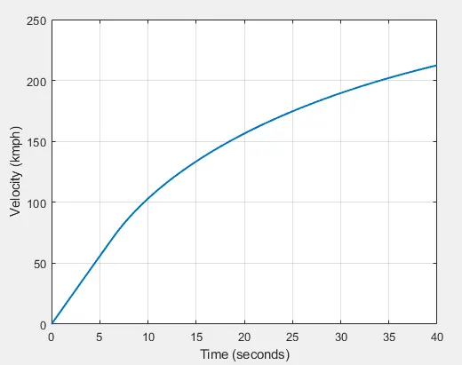
The Plot obatined by considering the original parameters:

The Plot obatined by changing the vehicle parameters:

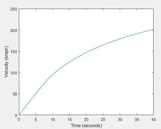
Conclusion:

The vehicle's acceleration reduces if the parameters of vehicle are increased by 5%.