Week 9 - Parametric study on Gate valve.

Parametric Study on Gate Valve

Aim: For this challenge, you will have to perform a parametric study on the gate valve simulation by setting the opening from 10 % to 80%.

• Obtain the mass flow rates at the outlet for each design point.
• Calculate the flow coefficient and flow factor for each opening and plot the graph.
• Discuss the results of the mass flow rate and flow coefficient.

Submit a well-defined report with all the necessary details.

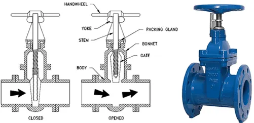
Theory: A gate valve, also known as a sluice valve, is a valve that opens by lifting a barrier (gate) out of the path of the fluid. Gate valves require very little space along the pipe axis and hardly restrict the flow of fluid when the gate is fully opened. The gate faces can be parallel but are most commonly wedge-shaped (in order to be able to apply pressure on the sealing surface).

Flow Coefficient: The flow coefficient of a device is a relative measure of its efficiency at allowing fluid flow. It describes the relationship between the pressure drop across an orifice valve or other assembly and, the corresponding flow rate. It is given by Cv,

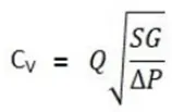
Where,

• Q = rate of flow (expressed in US Gallons per min)
• SG = Specific Gravity of the fluid (for water = 1)
• ∆P is the pressure drop across the valve (expressed in psi)

Flow Factor: The flow factor is the metric equivalent of flow coefficient (commonly used in Europe and Asia) and is calculated using metric units.

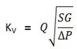
Where,

• Q = rate of flow (expressed in cubic meters per hour)
• SG = Specific Gravity of the fluid (for water = 1)
• ∆P is the pressure drop across the valve (expressed in bar)

K_v = 0.865 C_v

The K_v factor of a valve indicates the water flow in m3/h, at a pressure drop across the valve of 1bar when the valve is completely open.

Steps for Simulation:

• Open Spaceclaim and import the given STP file of the gate valve.

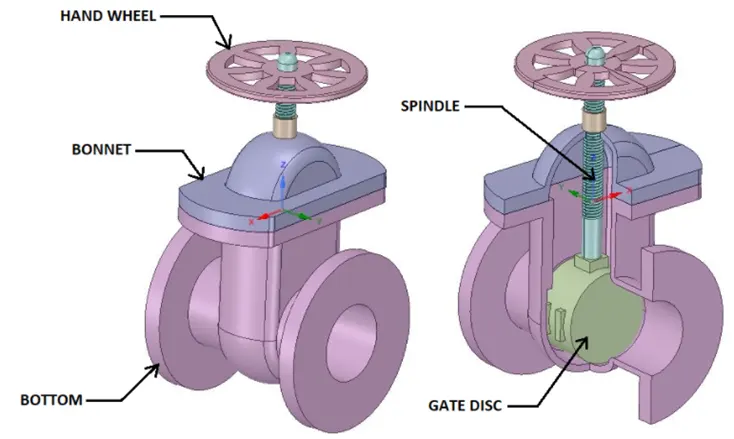
• Pull the faces of both inlet and outlet to 800mm each, respectively for convenience.
• Select “Gate Disc” and move the component upwards by 10mm (Z-direction).
• Notice the “P” symbol while editing/moving the component by 10mm, next to the dialogue box. This symbol is an option to parameterize the lift of the “Gate Disc”. Select it. The symbol turns grey. You also see a message stating “Group has been created” for lift.
• The lift value is now parameterized.
• Select 3 edges (inlet, outlet and upper edge of the part named “Bottom”) for the fluid volume.
• Suppress the 3D model for physics, as the analysis would be performed on the fluid volume only.

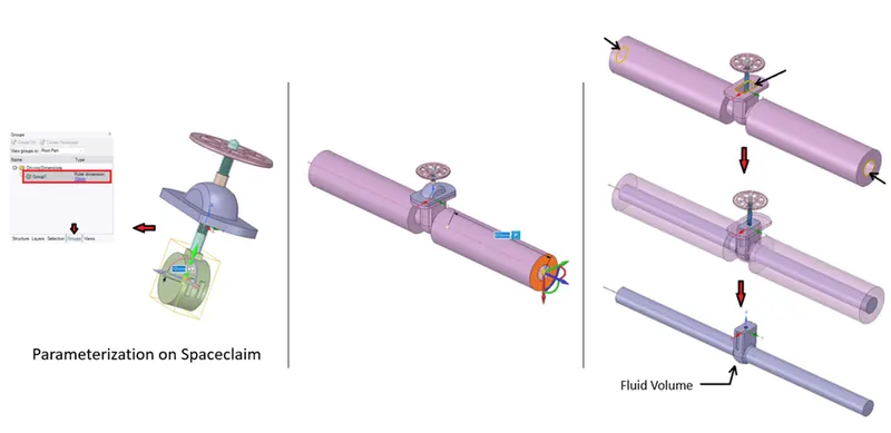
• Enter Mesh Module. Default mesh can be created. (elem size= 92.892mm)
• Create Named Selections for inlet and outlet of the fluid volume. Exit Mesh module.
• In Fluent module, choose steady state. Pressure based solver. Gravity = -9.81m/s².
• Material chosen = Water (liquid). Delete Air from the simulation for safety.
• Boundary Conditions:
  • Inlet type Pressure-inlet. Gauge pressure = 10 Pa.
  • Outlet Type Pressure outlet. Gauge pressure = 0 Pa.
  • Wall type- Wall. Stationary Wall. No Slip Condition
• Viscous Model = K-Epsilon (Realizable, Scalable Wall Functions). This is so because the flow is turbulent. We can get to know the flow is turbulent by the following calc.
  • To get to know the velocity of flow at inlet at 10 Pa, initialize the solution from Options--> Note down the Y component velocity.
  • 
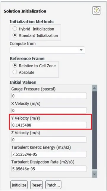
  • Density (ρ) = 998.2kg/m³. Velocity (V) = 0.1415488 m/s. Diameter (d) = 0.1m. Dynamic Viscosity (µ) = 0.001003 Ns/m².
  • Re = ρVD/µ. We get Re = 14087.14 > 2000. Hence the flow is turbulent.
• Create contours for velocity.
• Create report definitions for the report of mass flow rate at the outlet. (Area weighted Avg report) In the creation dialogue box, check report file, report plot and create output parameter.
• Initialize the solution.
• for 250 no. of iterations.
• After calculation is complete, exit fluent.
• In the workbench window we can see the Parameterization of Lift.
• Enter values from 20 to 80mm in the table. Check “Retain” in each row. Click update all Design Points.

Results:

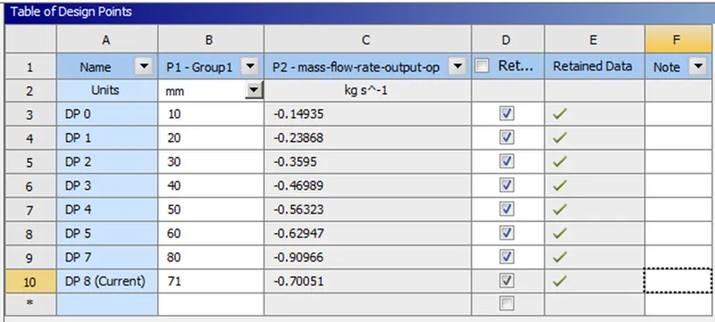
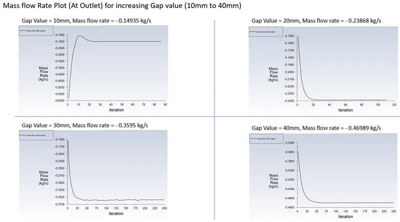
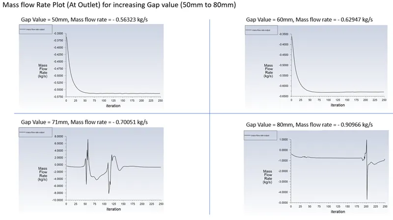
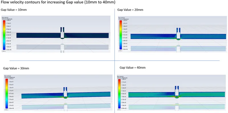
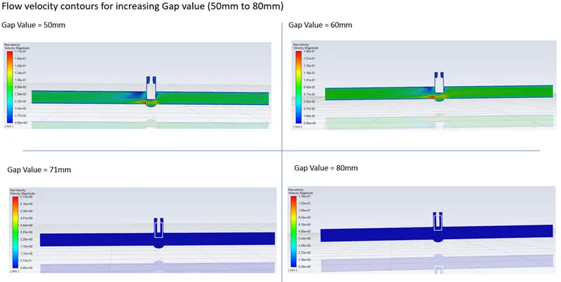
Mass Flow rates and plots at outlets for increasing gap values can be see in the images below. Negative mass flow rate value signifies that the flow is leaving the system or exiting through outlet.

Flow Factor & Flow Coefficient table:

Taking Pressure drop = 10 Pa as pressure at outlet is 0 and specific gravity = 1 (as the fluid is water) we get the following values:

Where, Flow coefficient is given by,

And Flow Factor = 0.865 * Flow coefficient

Conclusion:

• Velocity in the first case is really low as the gate disc opening is only 10mm high. As the gate opening increases the flow velocity also increases.
• The pressure at the outlet drops to 0 from 10Pa at the inlet because there are no restrictions/obstacles.
• Parameterizing the gate disc opening has enabled us to find the mass flow rate values quickly. It has saved significant time.