Week 8 - Simulating Cyclone separator with Discrete Phase Modelling

Cyclone Separator Simulation

Aim: To perform analysis on cyclone separator and calculate the separation efficiency and pressure drop.

• Write a few words about any four empirical models used to calculate the cyclone separator efficiency.
• Case 1: Perform an analysis on a given cyclone separator model by varying the particle diameter from 1 μm to 5 μm and calculate the separation efficiency in each case. Discuss the results. [Use both the velocity's as 3m/sec.]
• Case 2: Perform an analysis on a given cyclone separator model by varying the particle velocity from 1 m/sec to 5 m/sec and calculate the separation efficiency and pressure drop in each case. Discuss the results. [Use particle diameter size as 5 μm for all cases & keep flow velocity same as particle velocity]

Boundary Conditions:

• Inlet and wall: Reflect
• Outlet (Top): Escape
• Outlet (Bottom/dustbin): Trap

Note: Structural mesh gives the best results, so you can use cut cell meshing approach available in Ansys Meshing.

Theory:

Cyclone separators are devices that use the principle of inertia to remove particulate matter from flue gases. Cyclone separators work much like a centrifuge, but with a continuous feed of dirty air. In a cyclone separator, dirty flue gas is fed into a chamber. The inside of the chamber creates a spiral vortex, similar to a tornado. This spiral formation and the separation are shown in the figure below. The lighter components of this gas have less inertia, so it is easier for them to be influenced by the vortex and travel up it. Contrarily, larger components of particulate matter have more inertia and are not as easily influenced by the vortex.

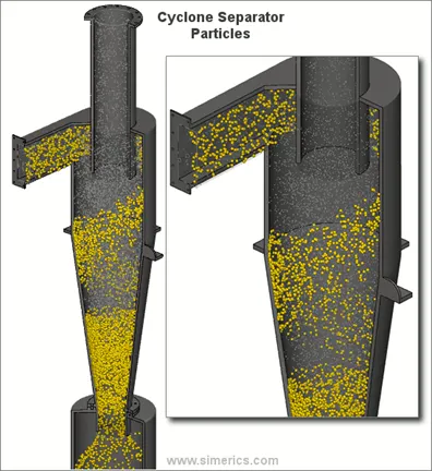
Since these larger particles have difficulty following the high-speed spiral motion of the gas and the vortex, the particles hit the inside walls of the container and drop down into a collection hopper. These chambers are shaped like an upside-down cone to promote the collection of these particles at the bottom of the container. The cleaned flue gas escapes out the top of the chamber.

Models to predict the behavior of cyclones are usually empirical. It remains, largely, a process of trial and error since empirical cyclone models are only applicable to specific cyclone geometries. Following four models have been described with brief introduction about them.

1) Lozia and Leith Model: Lozia and Leith logistic model is a modified version of Barth model which is developed based on force balance. The model assumes that a particle carried by the vortex endures the influence of two forces: a centrifugal force and a flow resistance.

The addition made by Lozia and Leith on the original Barth (1956) model are the core length and slope parameter expression which is derived based on the statistical analysis of experimental data of cyclone with D = 0.25 m.

2) Li & Wang Model: The Li and Wang (1989) model includes particle bounce or re-entrainment and turbulent diffusion at the cyclone wall. A two-dimensional analytical expression of particle distribution in the cyclone is obtained.

3) Koch & Licht Model: Koch and Licht collection theory recognized the inherently turbulent nature of cyclones and the distribution of gas residence times within the cyclone. Koch and Licht describe particle motion in the entry and collection regions.

4) Lapple Model: Lapple model was developed based on force balance without considering the flow resistance. Lapple assumed that a particle entering the cyclone is evenly distributed across the inlet opening. The particle that travels from inlet half width to the wall in the cyclone is collected with 50% efficiency.

Steps for Simulation:

• Import the given 3D model of the cyclone separator into SpaceClaim.
• Extract the fluid volume. Suppress the original 3D model for physics. Exit Spaceclaim.
• Open Mesh module. Assign tetramesh method of meshing to the fluid volume model. Overall mesh size = 8mm.
• Assign named selections – Inlet, Walls, Outlet Top and Outlet dustbin. Exit Mesh module.
• Open Fluent. The following is set in Fluent:
  • Pressure based, Steady State Condition. Gravity = -9.81m/s² in Y-axis.
  • Viscous model: K-epsilon (RNG model with swirl dominated flow)
  • DPM (Discrete Phase Modelling): Considering Coupled flow. Interactions with continuous phase and update DPM sources every flow iteration (10 intervals).
    • Injections = Anthracite (material). Particle type = Inert
    • X-Velocity of injection = Inlet velocity of air = Depends on case
    • Diameter of Particle = Depends on Case
  • In Case 1: Keep Inlet flow velocity = Particle Velocity = 3m/s. Vary particle diameter: 1 μm, 3 μm, 5 μm
  • In Case 2: Keep Particle Diameter = 5 μm, vary inlet flow velocity = particle velocity = 1m/s, 3m/s, 5m/s
  • Boundary Conditions:
    • Inlet = Velocity (Depends on Case). DPM = Reflect (Given)
    • Outlet dustbin- DPM = Trap (Given)
    • Outlet Top- DPM = Escape (Given)
    • Wall- DPM = Reflect (Given)
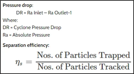
  • To calculate Pressure-drop, the pressure has been calculated at the inlet & top outlet condition.
  • (After calculation results, Reports--> Surface Integrals --> Area-weighted average --> Static Pressure --> Inlet/Outlet) The total pressure will be measured at both points and the drop in pressure will be calculated by deducting the outlet pressure from inlet pressure.
  • Also calculate Separator Efficiency.

• Standard Initialization. Initialise with Options --> Compute From --> Inlet
• No of iterations = 600.

Results:

Case 1: Keep Inlet flow velocity = Particle Velocity = 3m/s. Vary particle diameter: 1 μm, 3 μm, 5 μm

• Run 1: Particle Diameter = 1 μm; Inlet Airflow Velocity = Particle Velocity = 3m/s

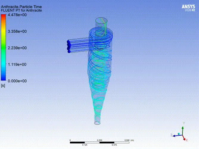
• Run 2: Particle Diameter = 3 μm; Inlet Airflow Velocity = Particle Velocity = 3m/s

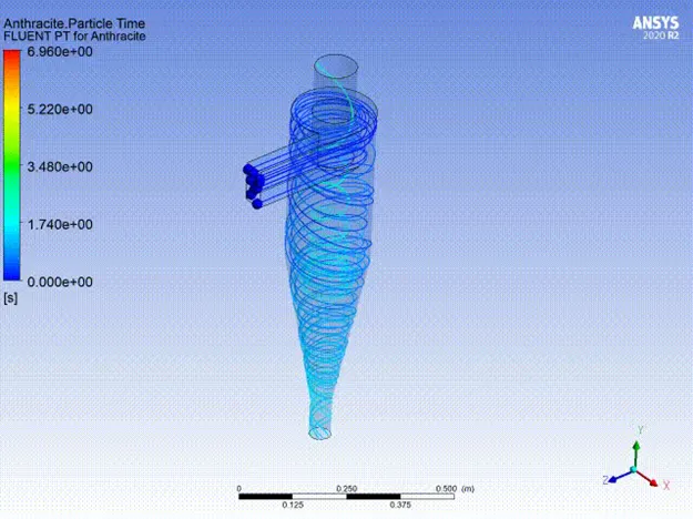
• Run 3: Particle Diameter = 5 μm; Inlet Airflow Velocity = Particle Velocity = 3m/s

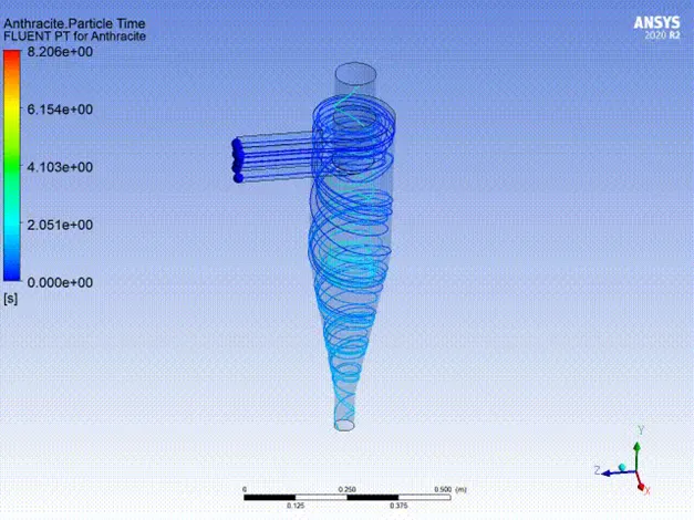
Case 2: Keep Particle Diameter = 5 μm, vary inlet flow velocity = particle velocity = 1m/s, 3m/s, 5m/s

• Run 1: Particle Diameter = 5 μm; Inlet Airflow Velocity = Particle Velocity = 1m/s

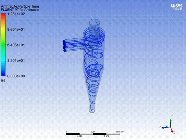
• Run 2: Particle Diameter = 5 μm; Inlet Airflow Velocity = Particle Velocity = 3m/s

• Run 3: Particle Diameter = 5 μm; Inlet Airflow Velocity = Particle Velocity = 5m/s

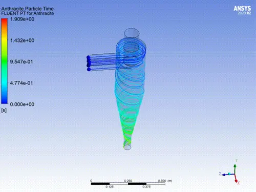
Conclusion:

Case 1: From the results, it can be observed that the separator efficiency increases with increasing particle diameter. This is because bigger particles have more mass. Larger components of particulate matter have more inertia and are not as easily influenced by the vortex, and therefore drop to the collector bin. The pressure at the outlet (on top) almost completely drops to 0. Therefore, the pressure drop observed = pressure at inlet. For all runs, the pressure drop is constant.

Case 2: From the results, it can be observed that the separator efficiency increases with increase in inlet velocity as well. This is because increase in velocity means increase in kinetic energy and more inertia. The outlet pressure (on top) drops to 0 once again. The pressure drop is as high as the inlet pressure. The pressure drop increases with increase in inlet pressure.