Week 9 - FVM Literature Review

FINITE VOLUME METHOD -

The finite volume is a discretisation method which is well suited for numerical simulations of various types namely hyperbolic, elliptic and parabolic for instance of conservation laws. It has been extensively used in several engineering fields, such as fluid mechanics, heat and mass transfer or petroleumengineering. Some of the important features of the finite volume metod are similar to those of finite element method. it may be used on arbitrary geometry using unstructured or structured meshes and it leads to robust schemes, another feature is local conservitivity of the numerical fluxes that is numerical flux is conserved from one discretisation cell to its neighbour.

DIFFERENCE BETWEEN FVM AND FDM-

The principle of Finite DIfference Method is, given a number of discretization points which may be defined by a mesh, to assign one discrete unknown per discretization point, and to write one equation per discretization points . At each discretization point the derivatives of the unknown are replaced by finite difference through the use of Taylor expansions.The finite difference method becomes difficult to use when the coefficients involved in the equation are discontinuous.With the finite vlolume method , discontinuous of the coefficients involved will not be any problem if the mesh is chosen such that the discontinuities of the coefficients occur on the boundaries of the control boundaries ."The finite volume schemes is also called cell centered difference scheme". Indeed in the finite volume method the finite difference approach can be used for  the approximation of the fluxes on the boundary of the control volume. 

Lets consider the 1D heat conduction equation

`del/(delx)(alpha(delT)/(delx))+s=0`

using the FDM method

 the equation is discretized and solved at each and every point.

limitations is that for an irregular surface it gets complicated to solve the problem.

FVM

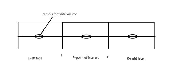
In case of FVM instead of writing the equation for points we consider volumes. Inside the particular  volume is for the flow is conserved flow quantities are conserved , energy is onserved flow quantities are conserved, energy is conserved mass is conserved, mass is conserved, momentum is conserved, which starts with ' integral form of governing equation'. 

Steps in FV discretization

1. Obtain the governing equation in its integral form.

2. Apply Gauss Divergence theorm.

3. Come up with suitable methods to calculate flux

Lets consider the 1D heat conduction equation

`del/(delx)(alpha(delT)/(delx))+S=0`

multiplying the governing wuation by 'dv' and integrating it

`int(del/(delx)(alpha(delT)/(delx))+S)dv=0`

`intdel/(delx)(alpha(delT)/(delx))dv+intSdv=0`

`intdel/(delx)(alpha(delT)/(delx))Adx+intSdv=0`

since `dv=A*dx`

`(alpha(delT)/(delx))Adx+barSdv=0`

`(alpha(delT)/(delx))A+barSdv=0`

 `alphaA((T_l-T_p)/(Deltax))-alphaA((T_p-T_r)/(Deltax))+barSdv=0`

NOTE:- if the source term added is the function of temperature we have to linearize it

Heat flux out -Heat flux in +source term=0

Interpolation scheme

The approximations of surface and volume integrals and volume integrals require values of the variables at locations other than computational nodes of the control volume .Values of these locations are obtained using interpolation formula.

Types 

1. Upwind interpolation.

2. Linear interpolation. 

3. Quadratic upwind interpolation.

4. Total Variation Diminish.

5.Hybrid Scheme.

Flux Limiters 

In fluid dynamics problems described by PDE's use in high resolution schemes to eliminate the spurious oscillations that would have occured with high order spatial discretization schemes due to shocks, discontinuous or sharp changes in the solution domain with a point of inflexion. Useof flux limiters, together with an appropriate with a point of inflexion. Use of flux limiters, together with an appropriate high resolution schemes makes the solution total varation diminishing.

The main moto of flux limiters schemes is to limit the spatial derivatives to realistic values concerned with certain science and engineering problems that usually means physically realisable and meaningful values. They are used in highresolution schemes for solving problems described PDE's and is only considered or taken into account when sharp wave fonts are present. For smoothly changing waves, the flux limiters doesnot operate and can be represented by higher order approximation without any introduction of spurious oscillations.