


Courses by Software
Courses by Semester
Courses by Domain
Tool-focused Courses
Machine learning
POPULAR COURSES
Success Stories

Week 7 - Simulation of a 1D Super-sonic nozzle flow simulation using Macormack Method
AIM- Simulation of 1D supersonic nozzle flow simulation using Macormack method OBJECTIVES- 1. Steady-state distribution of primitive variables inside the nozzle2. Time-wise variation of the primitive variables3. Variation of Mass flow rate distribution inside the nozzle at different time steps during the time-marching…
Mainak Bhowmick
updated on 30 Sep 2020


AIM- Simulation of 1D supersonic nozzle flow simulation using Macormack method
OBJECTIVES-
1. Steady-state distribution of primitive variables inside the nozzle
2. Time-wise variation of the primitive variables
3. Variation of Mass flow rate distribution inside the nozzle at different time steps during the time-marching process
4. Comparison of Normalized mass flow rate distributions of both forms
THEORY
The steady ,isentropic flow through a convergent_divergent nozzle is considered.The flow at the inlet to the nozzle comes from a reservoir where the pressure and temperature are denoted by ρ0andT0ρ0andT0respectively.The area is large hence the velocity tends to zero. Thus the
ρ0andT0ρ0andT0are the stagnation values or the total pressure and total temperature respectively. The flow expands isentropically to supersonic speeds at the nozzle exit, where the exit pressure , temperature velocity and mach number are denoted byρe,Te,VeandMeρe,Te,VeandMerespectively. The flow is locally subsonic in the convergent section of the nozzle ,sonic at the throatand supersonic at the divergent section.
i.e. at M<1:subsonic
M=1:sonic
M>1:supersonic

FIG:-schematic diagram of supersonic- subsonic isentropic nozzle flow
GOVERNING EQUATIONS
Continuity:
ρ1V1A1=ρ2V2A2ρ1V1A1=ρ2V2A2
Momentum
ρ1V1A1+ρ1V21A1+∫A2A1p.dA=ρ2V2A2+ρ2V22A2ρ1V1A1+ρ1V21A1+∫A2A1p.dA=ρ2V2A2+ρ2V22A2
Energy
h1+V212=h2+V222h1+V212=h2+V222
SOLVING THE EQUATIONS ANALYTICALLY
AA⋅=1M2⋅[(2γ+1)⋅(1+γ-12⋅M2)]γ+1γ-1AA⋅=1M2⋅[(2γ+1)⋅(1+γ−12⋅M2)]γ+1γ−1
PP0=(1+γ-12⋅M2)-(γγ-1)PP0=(1+γ−12⋅M2)−(γγ−1)
ρρ0=(1+γ-12⋅M2)-(1γ-1)ρρ0=(1+γ−12⋅M2)−(1γ−1)
TT0=(1+γ-12⋅M2)-1TT0=(1+γ−12⋅M2)−1
TIME STEP USED FOR THE CODE
dt=c*(min(ΔXa+VΔXa+V))
NON CONSERVATIVE FORM OF EQUATION
CONTINUITY
∂ρ′A′∂t′+ρA′∂V′∂X′+ρ′V′∂A′∂X′+V′A′∂P′∂X′=0
MOMENTUM
ρ∂V′∂t′+ρV′∂V′∂X′=-R(ρ′∂T′∂X′+T′∂P′∂X′)
ENERGY
ρ′Cv∂T′∂t′+ρ′V′Cv∂T′∂X′=-ρ′RT′[∂V′∂X′+V′∂lnA′∂X′]
INPUTS
ρ=1-0.3146X
T=1-0.2314X
V=(0.1+1.09X)T12
CODE TO SOLVE NON CONSERVATIVE
function [rho, v, t, rho_t, v_t, t_t, M_t, p_t, m]=non_conservation(nt,n,x,gamma,c,a,dx,throat)


    %calculation initial profiles
    rho=1-0.3146*x;
    t=1-0.2314*x;
    v=(0.1+1.09*x).*t.^0.5;
    dt=min(c.*dx./(sqrt(t).*v));

  for k=1:nt
            rho_old=rho;
            t_old=t;
            v_old=v;


        %predictor method


        for j=2:n-1

            dvdx=(v(j+1)-v(j))/dx;
            drhodx=(rho(j+1)-rho(j))/dx;
            dtdx=(t(j+1)-t(j))/dx;
            dlogadx=(log(a(j+1))-log(a(j)))/dx;

            %continuity equation
            drhodt_p(j)=-rho(j)*dvdx-rho(j)*v(j)*dlogadx-v(j)*drhodx;

            %momentum equation
            dvdt_p(j)=-v(j)*dvdx-(1/gamma)*(dtdx+(t(j)/rho(j))*drhodx);

            %energy equation
            dtdt_p(j)=-v(j)*dtdx-(gamma-1)*t(j)*(dvdx+v(j)*dlogadx);

            %update
                   rho(j)=rho(j)+drhodt_p(j)*dt;
                   v(j)=v(j)+dvdt_p(j)*dt;
                   t(j)=t(j)+dtdt_p(j)*dt;

        end


        %corrector steps

         for j=2:n-1
            dvdx=(v(j)-v(j-1))/dx;
            drhodx=(rho(j)-rho(j-1))/dx;
            dtdx=(t(j)-t(j-1))/dx;
            dlogadx=(log(a(j))-log(a(j-1)))/dx;

            %continuity equation
            drhodt_c(j)=-rho(j)*dvdx-rho(j)*v(j)*dlogadx-v(j)*drhodx;

            %momentum equation
            dvdt_c(j)=-v(j)*dvdx-(1/gamma)*(dtdx+(t(j)/rho(j))*drhodx);

            %energy equation
            dtdt_c(j)=-v(j)*dtdx-(gamma-1)*t(j)*(dvdx+v(j)*dlogadx);


         end
        %average time derivative
        drhodt=0.5*(drhodt_c+ drhodt_p);
        dvdt=0.5*(dvdt_c+dvdt_p);
        dtdt=0.5*(dtdt_c+dtdt_p);

        for i=2:n-1
        %final solution update
        v(i)=v_old(i)+dvdt(i)*dt;
        rho(i)=rho_old(i)+drhodt(i)*dt;
        t(i)=t_old(i)+dtdt(i)*dt;
        end

        %boundar conditions
        %input
        v(1)=2*v(2)-v(3);

        %output
        v(n)=2*v(n-1)-v(n-2);
        rho(n)=2*rho(n-1)-rho(n-2);
        t(n)=2*t(n-1)-t(n-2);

        %defining pressure mass flow and mach number
        p=rho.*t;
        m=rho.*a.*v;
        M=v./sqrt(t);


        %for the throat
        t_t(k)=t(throat);
        p_t(k)=p(throat);
        rho_t(k)=rho(throat);
        v_t(k)=v(throat);
        M_t(k)=M(throat);
        m(k,:)=m(throat);

     %plotting non dimensional distance vs mass
     figure(1)
       hold on
           if k==50
                plot(x,m,'b')
           elseif k==100
                plot(x,m,'g')
           elseif k==150
                plot(x,m,'y')
           elseif k==200
                plot(x,m,'m')
           elseif k==700
                plot(x,m,'c')
                legend('50','100','150','200','700')
                xlabel('nondimensional distance through nozzle')
                ylabel('mass flow rate')
          end


  end

  %plotting the time step non dimensional parameters
     figure(2)
        subplot(4,1,1)
        plot(p_t,'m');
        ylabel('P/P0');
        subplot(4,1,2)
        plot(t_t,'g');
        ylabel('T/T0');
        subplot(4,1,3)
        plot(rho_t,'b')
        ylabel('Density/Density0');
        subplot(4,1,4)
       % plot(M_throat,'r')
        ylabel('Mlabel');
        xlabel('no of time steps');

  %plotting non dimensional distance vs mass
     figure(3)
        subplot(4,1,1)
        plot(x,M,'b')
        axis([0 3 0 4])
       ylabel('Mach Number');
        grid on;
        subplot(4,1,2)
        plot(x,p,'g');
        axis([0 3 0 1.2])
        ylabel('Pressure ratio');
         grid on;
        subplot(4,1,3)
        plot(x,rho,'r');
        axis([0 3 0 1.2])
        ylabel('density ratio');
         grid on;
        subplot(4,1,4)
        plot(x,t,'m');
        axis([0 3 0 1.2])
        ylabel('temperature');
        xlabel('X');
        grid on;
end
OUTPUT
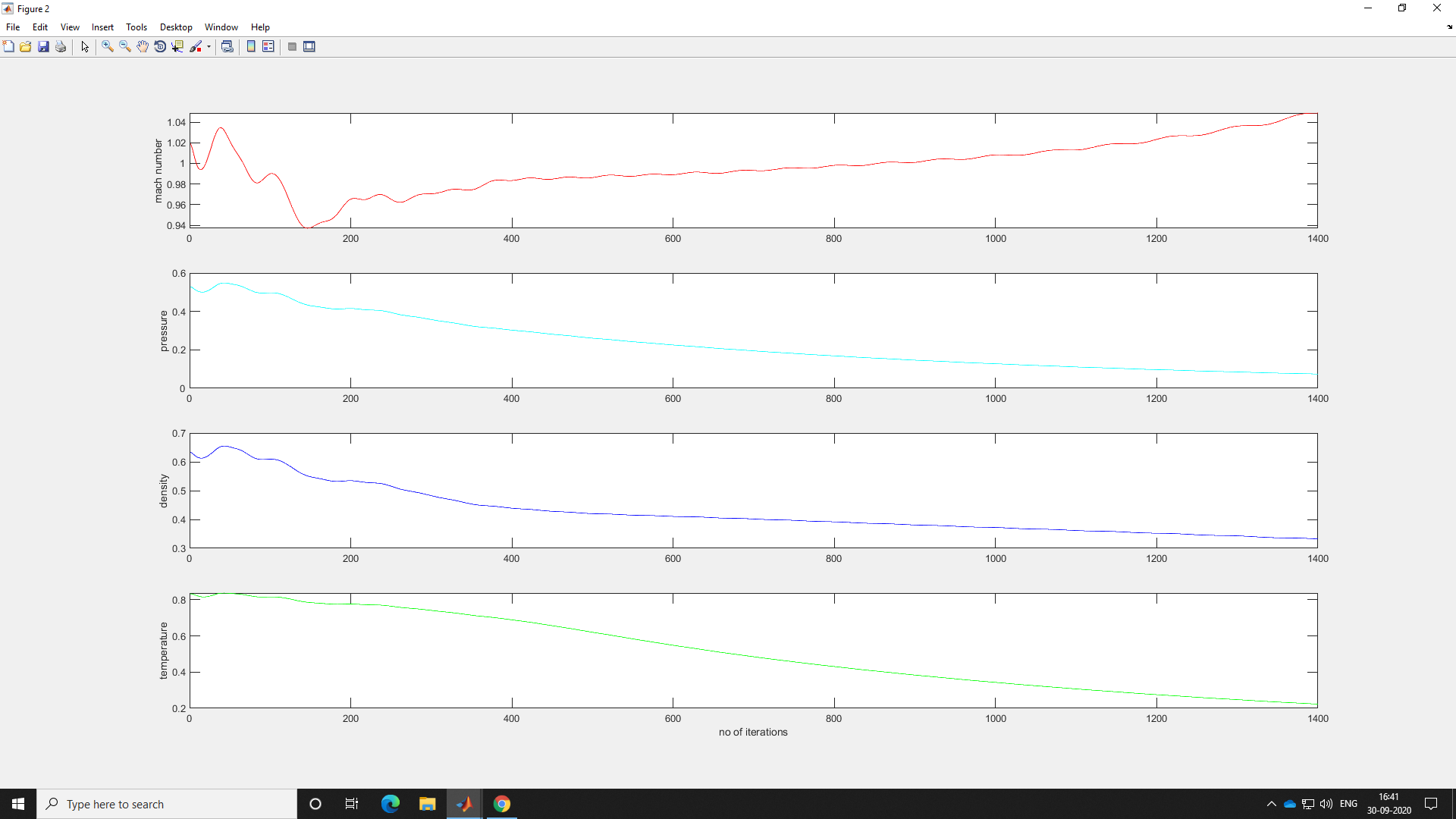
QUALiTATIVE ASPECTS

Time wise variation of density machnumber pressure and temperature

NON DIMENSIONAL DISTANCE VS MASS FLOW RATE FOR DIFFERENT TIME STEP

CONSERVATIVE EQUATIONS
CONTINUITY
∂ρ′A′∂t′+∂ρ′A′∂x=0
MOMENTUM
∂ρ′A′V′∂t+∂[ρ′A′V′2+1γρ′A′)∂X=1γP′∂A′∂V′
ENERGY
∂(ρ′(e′γ-1+γ2V′2)A′)∂t′+∂ρ′(e′γ-1+γ2V′2)∂X′V′A′+ρ′A′V′=0
TO SOLVE THE EQUATIONS WE CONSIDER
U1=ρ′A′
U2=ρ′A′V′
U3=ρ′(e′γ-1+γ2V′2)A
f1=ρ′A′V′
f2=ρ′A′V′+1γρ′A′
f3=ρ′(e′γ-1+γ2V′2)V′A′+p′A′V′
J=1γρ′∂A′∂x′
FINAL EQUATIONS
∂U1∂(t′)=-∂F1∂X′
∂U2∂(t′)=-∂F2∂X′+J2
∂U3∂(t′)=-∂F3∂X′
INITIAL CONDITIONS
ρ′=1.0;T′=1.0-{0≤X′≤0.5}
ρ′=1.0-0.366(X′-0.5);T′=1.0-0.167(X′-0.5)-{0.5≤X′≤1.5}
ρ′=0.634-0.3879(X′-1.5);T′=0.833-0.3507(X′-1.5)-{1.5≤X′≤3.5}
function [rho, v, t,rho_th,v_th,t_th,M_th, p_th,m_th]=conservation(nt,n,x,gamma,c,a,dx,throat)


    %initial values
    for i=1:n
        if (x(i)>=0 && x(i)<=0.5)
         rho(i)=1;
         t(i)=1;

        elseif (x(i)>=0.5 && x(i)<=1.5)
         rho(i)=1-0.366*(x(i)-0.5);
         t(i)=1-0.167*(x(i)-0.5);

      elseif (x(i)>=1.5 && x(i)<=3.5)
        rho(i)=0.634-0.3879*(x(i)-1.5);
        t(i)=0.8355-0.3507*(x(i)-1.5);
        end
    end

    v=0.59./(rho.*a);
    %timr step
    dt=min(c.*dx./(sqrt(t)+v));

    %Mackmorks technique for solving
    U_1=rho.*a;
    U_2=rho.*a.*v;
    U_3=rho.*a.*((t./(gamma-1))+((gamma./2).*(v.^2)));


    %time loop
    for k=1:nt


       U_old1=U_1;
       U_old2=U_2;
       U_old3=U_3;


        f1=U_2;
        f2=((U_2.^2)./U_1)+(((gamma-1)/gamma)*(U_3-((gamma/2)*((U_2.^2)./U_1))));
        f3=((gamma*U_2.*U_3)./U_1)-(gamma*(gamma-1)*(U_2.^3))./(2*(U_1.^2));


        %predictor step
        for j=2:n-1
         dadx=((a(j+1)-a(j)))/dx;
         J2=rho(j)*t(j)*dadx/gamma;

         %continuity equation
         dudt1p(j)=-(f1(j+1)-f1(j))/dx;

         %momentum equation
         dudt2p(j)=-(f2(j+1)-f2(j))/dx+J2;

         %energy
         dudt3p(j)=-(f3(j+1)-f3(j))/dx;

         %solution update
            U_1(j)=U_1(j)+ dudt1p(j)*dt;
            U_2(j)=U_2(j)+ dudt2p(j)*dt;
            U_3(j)=U_3(j)+ dudt3p(j)*dt;

        end

        %Decoding the values
        rho_p=U_1./a;
        v_p=U_2./U_1;
        t_p=(gamma-1)*((U_3./U_1)-((gamma/2)*(v_p.^2)));
        v_p=U_2./U_1;
        f1=U_2;
        f2=((U_2.^2)./U_1)+(((gamma-1)/gamma)*(U_3-((gamma/2)*((U_2.^2)./U_1))));
        f3=((gamma*U_2.*U_3)./U_1)-(gamma*(gamma-1)*(U_2.^3))./(2*(U_1.^2));


     for j=2:n-1

            dadx=((a(j)-a(j-1)))/dx;
            J2=rho_p(j).*t_p(j).*dadx/gamma;

         %continuity equation
         dudt1c(j)=-(f1(j)-f1(j-1))/dx;

         %momentum equation
         dudt2c(j)=-(f2(j)-f2(j-1))/dx+J2;

         %energy
         dudt3c(j)=-(f3(j)-f3(j-1))/dx;


     end

     %average time step
     dudt1=0.5*(dudt1p+dudt1c);
     dudt2=0.5*(dudt2p+dudt2c);
     dudt3=0.5*(dudt3p+dudt3c);

     %final solution
     for i=1:n-1
         U_1(i)=U_old1(i)+dudt1(i)*dt;
         U_2(i)=U_old2(i)+dudt2(i)*dt;
         U_3(i)=U_old3(i)+dudt3(i)*dt;

    end

    %boundary conditions

    %inlet
    U_1(1)=rho_p(1).*a(1);
    U_2(1)=2*U_2(2)-U_2(3);
    v_p(1)=U_2(1)/U_1(1);
    U_3(1)=U_1(1)*((t_p(1)/(gamma-1))+((gamma/2)*v_p(1).*v_p(1)^2));

    %outlet
    U_1(n)=2*U_1(n-1)-U_1(n-2);
    U_2(n)=2*U_2(n-1)-U_2(n-2);
    U_3(n)=2*U_3(n-1)-U_3(n-2);


    %primitive variables decoding
    rho=U_1./a;
    v=U_2./U_1;
    t=(gamma-1)*((U_3./U_1)-((gamma/2)*(v.^2)));
    M=v./((t).^0.5);
    p=rho.*t;
    m(k,:)=rho.*v.*a;

    %values at thrust
    rho_th(k)=rho(throat);
    v_th(k)=v(throat);
    t_th(k)=t(throat);
    M_th(k)=M(throat);
    p_th(k)=p(throat);
    m_th(k)=m(throat);


end
    %plotting the time step non dimensional parameters
    figure(1)
    subplot(4,1,1)
    plot(x,M,'r')
    ylabel('Mach number')
    subplot(4,1,2)
    plot(x,p,'b')
    ylabel('pressure')
    subplot(4,1,3)
    plot(x,rho,'c')
    ylabel('density')
    subplot(4,1,4)
    plot(x,t,'g')
    ylabel('temperature')
    xlabel('X')


    %plotting non dimensional distance vs mass
    figure(2)
    subplot(4,1,1)
    plot(M_th,'r')
    ylabel('mach number')
    subplot(4,1,2)
    plot(p_th,'c')
    ylabel('pressure')
    subplot(4,1,3)
    plot(rho_th,'b')
    ylabel('density')
    subplot(4,1,4)
    plot(t_th,'g')
    ylabel('temperature')
    xlabel('no of iterations')
end
OUTPUT

MAIN PROGRAM
clear all
close all
clc

%grid points
value_of_n=input('1 for 31 2 for 61:' );
if value_of_n==1
    n=31;
elseif value_of_n==2
    n=61;
end
%Length of
x=linspace(0,3,n);
dx=x(2)-x(1);
gamma=1.4;
c=.5;


a=1+2.2*(x-1.5).^2;
throat=(n+1)/2;
%time steps
nt=1400;

[rho_n, v_n, t_n, rho_th_n, v_th_n, t_th_n, M_th_n, p_th_n, m_n]=non_conservation(nt,n,x,gamma,c,a,dx,throat);
[rho_c, v_c, t_c, rho_th_c, v_th_c, t_th_c, M_th_c, p_th_c, m_c]=conservation(nt,n,x,gamma,c,a,dx,throat);
CALCULATING MASS FLOW WRT X
function [rho, v, t, rho_t, v_t, t_t, M_t, p_t, m_t,m]=non_conservation(nt,n,x,gamma,c,a,dx,throat)


    %calculation initial profiles
    rho=1-0.3146*x;
    t=1-0.2314*x;
    v=(0.1+1.09*x).*t.^0.5;
    dt=min(c.*dx./(sqrt(t).*v));

  for k=1:nt
            rho_old=rho;
            t_old=t;
            v_old=v;


        %predictor method


        for j=2:n-1

            dvdx=(v(j+1)-v(j))/dx;
            drhodx=(rho(j+1)-rho(j))/dx;
            dtdx=(t(j+1)-t(j))/dx;
            dlogadx=(log(a(j+1))-log(a(j)))/dx;

            %continuity equation
            drhodt_p(j)=-rho(j)*dvdx-rho(j)*v(j)*dlogadx-v(j)*drhodx;

            %momentum equation
            dvdt_p(j)=-v(j)*dvdx-(1/gamma)*(dtdx+(t(j)/rho(j))*drhodx);

            %energy equation
            dtdt_p(j)=-v(j)*dtdx-(gamma-1)*t(j)*(dvdx+v(j)*dlogadx);

            %update
                   rho(j)=rho(j)+drhodt_p(j)*dt;
                   v(j)=v(j)+dvdt_p(j)*dt;
                   t(j)=t(j)+dtdt_p(j)*dt;

        end


        %corrector steps

         for j=2:n-1
            dvdx=(v(j)-v(j-1))/dx;
            drhodx=(rho(j)-rho(j-1))/dx;
            dtdx=(t(j)-t(j-1))/dx;
            dlogadx=(log(a(j))-log(a(j-1)))/dx;

            %continuity equation
            drhodt_c(j)=-rho(j)*dvdx-rho(j)*v(j)*dlogadx-v(j)*drhodx;

            %momentum equation
            dvdt_c(j)=-v(j)*dvdx-(1/gamma)*(dtdx+(t(j)/rho(j))*drhodx);

            %energy equation
            dtdt_c(j)=-v(j)*dtdx-(gamma-1)*t(j)*(dvdx+v(j)*dlogadx);


         end
        %average time derivative
        drhodt=0.5*(drhodt_c+ drhodt_p);
        dvdt=0.5*(dvdt_c+dvdt_p);
        dtdt=0.5*(dtdt_c+dtdt_p);

        for i=2:n-1
        %final solution update
        v(i)=v_old(i)+dvdt(i)*dt;
        rho(i)=rho_old(i)+drhodt(i)*dt;
        t(i)=t_old(i)+dtdt(i)*dt;
        end

        %boundar conditions
        %input
        v(1)=2*v(2)-v(3);

        %output
        v(n)=2*v(n-1)-v(n-2);
        rho(n)=2*rho(n-1)-rho(n-2);
        t(n)=2*t(n-1)-t(n-2);

        %defining pressure mass flow and mach number
        p=rho.*t;
        m(k,:)=rho.*a.*v;
        M=v./sqrt(t);


        %for the throat
        t_t(k)=t(throat);
        p_t(k)=p(throat);
        rho_t(k)=rho(throat);
        v_t(k)=v(throat);
        M_t(k)=M(throat);
        m_t(k)=m(throat);


end
function [rho, v, t,rho_th,v_th,t_th,M_th, p_th,m_th,m]=conservation(nt,n,x,gamma,c,a,dx,throat)
%initial values
for i=1:n
if (x(i)>=0 && x(i)<=0.5)
rho(i)=1;
t(i)=1;
elseif (x(i)>=0.5 && x(i)<=1.5)
rho(i)=1-0.366*(x(i)-0.5);
t(i)=1-0.167*(x(i)-0.5);
elseif (x(i)>=1.5 && x(i)<=3.5)
rho(i)=0.634-0.3879*(x(i)-1.5);
t(i)=0.8355-0.3507*(x(i)-1.5);
end
end
v=0.59./(rho.*a);
%timr step
dt=min(c.*dx./(sqrt(t)+v));
%Mackmorks technique for solving
U_1=rho.*a;
U_2=rho.*a.*v;
U_3=rho.*a.*((t./(gamma-1))+((gamma./2).*(v.^2)));
%time loop
for k=1:nt
U_old1=U_1;
U_old2=U_2;
U_old3=U_3;
f1=U_2;
f2=((U_2.^2)./U_1)+(((gamma-1)/gamma)*(U_3-((gamma/2)*((U_2.^2)./U_1))));
f3=((gamma*U_2.*U_3)./U_1)-(gamma*(gamma-1)*(U_2.^3))./(2*(U_1.^2));
%predictor step
for j=2:n-1
dadx=((a(j+1)-a(j)))/dx;
J2=rho(j)*t(j)*dadx/gamma;
%continuity equation
dudt1p(j)=-(f1(j+1)-f1(j))/dx;
%momentum equation
dudt2p(j)=-(f2(j+1)-f2(j))/dx+J2;
%energy
dudt3p(j)=-(f3(j+1)-f3(j))/dx;
%solution update
U_1(j)=U_1(j)+ dudt1p(j)*dt;
U_2(j)=U_2(j)+ dudt2p(j)*dt;
U_3(j)=U_3(j)+ dudt3p(j)*dt;
end
%Decoding the values
rho_p=U_1./a;
v_p=U_2./U_1;
t_p=(gamma-1)*((U_3./U_1)-((gamma/2)*(v_p.^2)));
v_p=U_2./U_1;
f1=U_2;
f2=((U_2.^2)./U_1)+(((gamma-1)/gamma)*(U_3-((gamma/2)*((U_2.^2)./U_1))));
f3=((gamma*U_2.*U_3)./U_1)-(gamma*(gamma-1)*(U_2.^3))./(2*(U_1.^2));
for j=2:n-1
dadx=((a(j)-a(j-1)))/dx;
J2=rho_p(j).*t_p(j).*dadx/gamma;
%continuity equation
dudt1c(j)=-(f1(j)-f1(j-1))/dx;
%momentum equation
dudt2c(j)=-(f2(j)-f2(j-1))/dx+J2;
%energy
dudt3c(j)=-(f3(j)-f3(j-1))/dx;
end
%average time step
dudt1=0.5*(dudt1p+dudt1c);
dudt2=0.5*(dudt2p+dudt2c);
dudt3=0.5*(dudt3p+dudt3c);
%final solution
for i=1:n-1
U_1(i)=U_old1(i)+dudt1(i)*dt;
U_2(i)=U_old2(i)+dudt2(i)*dt;
U_3(i)=U_old3(i)+dudt3(i)*dt;
end
%boundary conditions
%inlet
U_1(1)=rho_p(1).*a(1);
U_2(1)=2*U_2(2)-U_2(3);
v_p(1)=U_2(1)/U_1(1);
U_3(1)=U_1(1)*((t_p(1)/(gamma-1))+((gamma/2)*v_p(1).*v_p(1)^2));
%outlet
U_1(n)=2*U_1(n-1)-U_1(n-2);
U_2(n)=2*U_2(n-1)-U_2(n-2);
U_3(n)=2*U_3(n-1)-U_3(n-2);
%primitive variables decoding
rho=U_1./a;
v=U_2./U_1;
t=(gamma-1)*((U_3./U_1)-((gamma/2)*(v.^2)));
M=v./((t).^0.5);
p=rho.*t;
m(k,:)=rho.*v.*a;
%values at thrust
rho_th(k)=rho(throat);
v_th(k)=v(throat);
t_th(k)=t(throat);
M_th(k)=M(throat);
p_th(k)=p(throat);
m_th(k)=m(throat);
end
clear all
close all
clc

%grid points
value_of_n=input('1 for 31 2 for 61:' );
if value_of_n==1
    n=31;
elseif value_of_n==2
    n=61;
end
%Length of
x=linspace(0,3,n);
dx=x(2)-x(1);
gamma=1.4;
c=.5;


a=1+2.2*(x-1.5).^2;
throat=(n+1)/2;
%time steps
nt=1400;

[rho_n, v_n, t_n, rho_th_n, v_th_n, t_th_n, M_th_n, p_th_n, m_n,mn]=non_conservation(nt,n,x,gamma,c,a,dx,throat);
[rho_c, v_c, t_c, rho_th_c, v_th_c, t_th_c, M_th_c, p_th_c, m_c,mc]=conservation(nt,n,x,gamma,c,a,dx,throat);

for i=1:nt
figure(1)
plot(x,mn(1,:),'b',x,mc(1,:),'r')
xlabel('X/L');
ylabel('mass flow rate')
end
OUTPUT

CONCLUSION
1. The conservative form does a better job in of preserving the mass throughout the flowfield.
2. Conservative requires more work.
3. The non conservative lower residuals.
Leave a comment
Thanks for choosing to leave a comment. Please keep in mind that all the comments are moderated as per our comment policy, and your email will not be published for privacy reasons. Please leave a personal & meaningful conversation.
Other comments...
Be the first to add a comment
Read more Projects by Mainak Bhowmick (6)
Week 11 - Simulation of Flow through a pipe in OpenFoam
AIM- Write a program in Matlab that can generate the computational mesh automatically for any wedge angle and grading schemes For a baseline mesh, show that the velocity profile matches with the Hagen poiseuille's equation Show that the velocity profile is fully developed Post process velocity and shear stress…

29 Oct 2020 06:38 PM IST
Week 9 - FVM Literature Review
FINITE VOLUME METHOD - The finite volume is a discretisation method which is well suited for numerical simulations of various types namely hyperbolic, elliptic and parabolic for instance of conservation laws. It has been extensively used in several engineering fields, such as fluid mechanics, heat and mass transfer or…
20 Oct 2020 10:43 AM IST
Week 8 - BlockMesh Drill down challenge
AIM-to create a BlockMesh and to simulate it . OBJECTIVES:- How does the velocity magnitude profile change as a function of mesh grading factor. Use factors, 0.2, 0.5,0.8 Measure the velocity profile at 0.085 m from the inlet of the geometry Plot must be a line plot Compare velocity magnitude contours near the step region…
15 Oct 2020 09:58 AM IST
Week 7 - Simulation of a 1D Super-sonic nozzle flow simulation using Macormack Method
AIM- Simulation of 1D supersonic nozzle flow simulation using Macormack method OBJECTIVES- 1. Steady-state distribution of primitive variables inside the nozzle2. Time-wise variation of the primitive variables3. Variation of Mass flow rate distribution inside the nozzle at different time steps during the time-marching…
30 Sep 2020 08:16 PM IST
Related Courses


0 Hours of Content
Skill-Lync offers industry relevant advanced engineering courses for engineering students by partnering with industry experts.


Our Company

4th Floor, BLOCK-B, Velachery - Tambaram Main Rd, Ram Nagar South, Madipakkam, Chennai, Tamil Nadu 600042.

Top Individual Courses
Top PG Programs
Skill-Lync Plus
Trending Blogs
© 2025 Skill-Lync Inc. All Rights Reserved.