Week 7 - Simulation of a 1D Super-sonic nozzle flow simulation using MacCormack Method

Solution 1D Super-sonic nozzle flow simulation using Macormack Method

AIM:

To simulate the isentropic flow through a quasi 1D subsonic-supersonic nozzle by solving the conservation and non-conservation forms of the governing equations using MacCormack's technique in MATLAB.

THEORY:

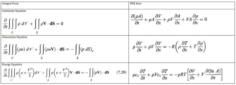
• In a comprehensive manner, first, we have to derive the PDE using the integral form of governing equation.
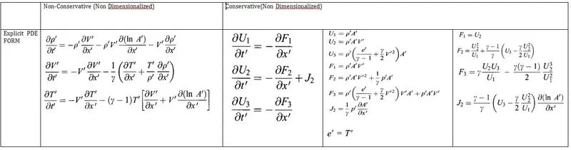
• Both non-conservative and conservative form of PDE is represented in a suitable form to get the explicit form of a difference equation.
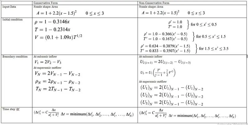
• Initial conditions are arbitrarily assumed, boundary conditions are specified after each time step and 'dt' is calculated based on CFL Condition.
• This difference equation is solved at each and every node at each time step till we get the steady-state solution.

PDE for nozzle:

• In real, nozzle flow is a 2D flow, because as the area changes with x, flow field variables changes in both x and y directions.
• Even though it is 2D, here it is assumed that flow variable vary only with x-direction, hence termed as quasi 1D nozzle flow.
• Hence, the general governing equation cannot be applied to this problem, first, we must use an integral form of governing equation, and these integral forms are applied to a control volume consistent with the quasi 1D assumption.
• We get a governing equation in both conservative and nonconservative PDE forms, both are mathematically equivalent, but from a numerical solution point of view, they are different.
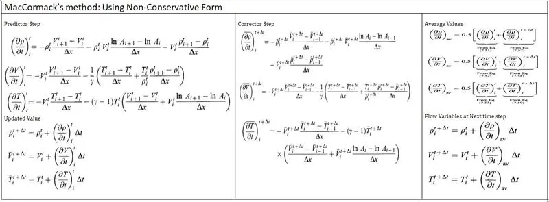
• Here both forms of PDE is discretized into difference equation using MacCormack's technique
• 
• 
• 

MacCormack's method:

• MacCormack's method consists of two main steps, predictor and corrector step.
• In the predictor step, the partial derivative with respect to space is discretized using the forward difference technique.
• Using predictor step value, flow variables values are updated for the next time step.
• In the corrector step, the partial derivative with respect to space is discretized using the backward difference technique.
• The updated values from the predictor step are used in the corrector step as an initial condition.
• The average value of flow variables from both steps is used to calculate flow variables at all discrete points at the next time step.
• These steps are repeated till a steady-state condition is achieved.

Nozzle Setup:

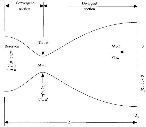
• The flow at the inlet to the nozzle comes from the reservoir since at the inlet reservoir area is large velocity is assumed to be zero.
• The flow expands isentropically to supersonic speed at the nozzle exit.
• At throat flow is Sonic, that is local velocity is equal to the local speed of sound.
• From an analytical solution point of view, Mach number is a function of area ratio, since the area is a function of x, Mach number also varies with x, similarly variation of pressure, density and temperature is a function of Mach number, it also varies with x (along with the nozzle in the X direction).
• For nozzle flow to happen, force must be exerted on gas to accelerate it through the nozzle, it is done by the pressure ratio across the nozzle. Since area changes pressure also changes hence the area ratio is designed in such a way that gives subsonic flow at convergent section and super Sonic flow at divergent section.
• At the subsonic inflow boundary, x = 0, two dependent flow field variables ( temperature and density) are independent of time, but the velocity is dependent on time, hence at every time step velocity at node 1 must be updated.
• At the supersonic outflow boundary, x =3m, all three flow variables are dependent on time, therefore their values are updated at each and every time step.
• 

Conservative and Non-conservative form Discretization setup:

• Initial and boundary conditions are different for conservative and non-conservative forms.
• The non-Conservative form of PDE is in terms of primitive flow variables and hence obtained solution is directly gives primitive variables value.
• In conservative form, the numerical solution does not directly give the solution of primitive flow field variables.
• The conservative form of PDE is expressed in terms of solution vector and flux vector, After solving, the solution vector is used to calculate primitive variables.
• While programming the Flux vector must be expressed in terms of the solution vector, otherwise, the solution becomes unstable.
• Here Discretization setup explained using the non-conservative form, same procedure is applied to the conservative form as well.
• 
• 

MATLAB CODE:

Main Code:

Filename: NozzleFlowBothForm

It asks input from the user Based on the user input, the code will either solve the problem using a non-conservative form of difference equation or a conservative form of a difference equation by calling a function. Through the function, we get two outputs. The first output gives the flow_variables, which is used to plot the steady-state distribution of primitive variables inside the nozzle. The second output gives the data, which is used to create a movie, to visualize the timewise variation of flow variables.

clear all
close all
clc

%% Discretization.

M = input('Enter 1 for conservative form and 2 for non conservative form: ');

%Length of nozzle
L = 3;

% Discretizated into 31 nodes
n = 31;

% Domain discretization in x direction
x = linspace(0,L,n);

% Discretization Length
dx = x(2)-x(1);

%number of time step
nt = 1400;
%% Inputs.

%Specific heat ration
gamma= 1.4;

%Nozzle Area
A = 1+(2.2*((x-1.5).^2));

%Courant number
C = 0.5;

%% Function to calculate Flow variable

if M == 1
[flow_variables,vid] = conservative(n,x,dx,A,gamma,C,nt);
NAME = 'ConservativeQuasiDNozzleFlow';
FORM = 'CONSERVATIVE FORM';
else
[flow_variables,vid] = nonconservative(n,x,dx,A,gamma,C,nt);
NAME = 'NonConservativeQuasiDNozzleFlow';
FORM = 'NonCONSERVATIVE FORM';
end
    
rho = (flow_variables(1,:));
V = (flow_variables(2,:));
temp = (flow_variables(3,:));

pressure = rho.*(temp);
Mach = V./((temp.^0.5));
Mass_Flow_Rate = rho.*V.*A;

%% To visualize The steady state Result
figure(1)
plot(x,rho)
xlabel('Nozzle length in x direction')
ylabel('Desnity')
title(FORM)
grid on
figure(2)
plot(x,V)
xlabel('Nozzle length in x direction')
ylabel('Velocity')
title(FORM)
grid on
figure(3)
plot(x,temp)
xlabel('Nozzle length in x direction')
ylabel('temperature')
title(FORM)
grid on
figure(4)
plot(x,(rho.*temp))
xlabel('Nozzle length in x direction')
ylabel('Pressure')
title(FORM)
grid on
figure(5)
plot(x,(rho.*V.*A))
xlabel('Nozzle length in x direction')
ylabel('Mass Flow Rate')
title(FORM)
grid on
figure(6)
plot(x,V./((temp.^0.5)))
xlabel('Nozzle length in x direction')
ylabel('Mach Number')
title(FORM)
grid on

%% to show time wise variation
movie(vid);
videofile = VideoWriter(NAME);
open(videofile);
writeVideo(videofile,vid);
close(videofile);

Function Code:

Filename: 1.conservative and 2.nonconservative

Both functions take the input from the main code. Initial Conditions are calculated based on the inputs. Necessary variables are defined to store the old values and frames. The first-time loop is defined, in a time loop at each time step, 'dt' is determined using another for loop. Within the time-loop, a space loop is defined, which calculates the variation of flow variables along the length of the nozzle. After each space loop, flow variables are calculated and boundary conditions are determined for next time step. After that flow parameters are plotted to get the frames to make a movie. OUTPUT = [FlowVariables,Frames]

Conservative

function [Flow_Variables,vid]= conservative(n,x,dx,A,gamma,C,nt)

%% Initial conditions as a function of x at time = 0sec.

for q =1:length(x)
    L = x(q);
    if (0<=L)&&(L<=0.5)
        rho(q) = 1;
        temp(q) = 1;
        V(q) = (0.59/(rho(q)*A(q)));
    elseif (0.5<=L)&&(L<=1.5)
        rho(q) = 1-(0.366*(x(q)-0.5));
        temp(q) = 1-(0.167*(x(q)-0.5));
        V(q) = (0.59/(rho(q)*A(q)));
    else
        rho(q) = 0.634-(0.3879*(x(q)-1.5));
        temp(q) = 0.833-(0.3507*(x(q)-1.5));
        V(q) = (0.59/(rho(q)*A(q)));
    end
end

%% conservative form solution
    U1 = rho.*A;
    U2 = rho.*A.*V;
    U3 = rho.*((temp/(gamma-1))+((gamma/2)*V.^2)).*A;
    F1 = U2;
    F2 = ((U2.^2)./U1)+(((gamma-1)/gamma)*(U3-((gamma/2)*((U2.^2)./U1))));
    F3_1 = (gamma*((U2.*U3)./(U1)));
    F3_2 = ((gamma*(gamma-1))/2)*((U2.^3)./(U1.^2));
    F3= F3_1-F3_2;
    
    frame = 1;
    
for time= 1:nt 
    
    time_step(1) = 1;
    for m = 1:n
        denominator = (temp(m)^0.5)+(V(m));
        time_step(m) = (C*dx)/denominator;
    end
    dt = min(abs(time_step));
    
    U1_old =U1;
    U2_old=U2;
    U3_old=U3;
    F1p = U2;
    F2p = ((U2.^2)./U1)+(((gamma-1)/gamma)*(U3-((gamma/2)*((U2.^2)./U1))));
    F3p_1 = (gamma*((U2.*U3)./(U1)));
    F3p_2 = ((gamma*(gamma-1))/2)*((U2.^3)./(U1.^2));
    F3p= F3p_1-F3p_2;
    
 %Boundary Conditions for next timestep at inlet
    U1(1) = rho(1)*A(1);
    U2(1) = (2*U2(2))-U2(3);
    V2(1) = U2(1)/U1(1);
    U3(1)  = U1(1)*((temp(1)/(gamma-1))+((gamma/2)*V2(1)^2));
    rho(1) = U1(1)/A(1);
    V(1) = U2(1)/U1(1);
    temp(1)=(gamma-1)*((U3(1)/U1(1))-((gamma/2)*V(1)^2));
    
    F1c(1) = U2(1);
    F2c(1) = ((U2(1)^2)/U1(1))+(((gamma-1)/gamma)*(U3(1)-((gamma/2)*((U2(1)^2)/U1(1)))));
    F3c_1 = (gamma*((U2(1)*U3(1))/(U1(1))));
    F3c_2 = ((gamma*(gamma-1))/2)*((U2(1)^3)/(U1(1)^2));
    F3c(1)= F3c_1-F3c_2;  
   
    for i = 2:n-1
        
        %Predictor step
        dF1_dx_p = (F1p(i+1)-F1p(i))/(dx);
        dF2_dx_p = (F2p(i+1)-F2p(i))/(dx);
        dF3_dx_p = (F3p(i+1)-F3p(i))/(dx);
        dA_dx_p = (A(i+1)-A(i))/(dx);
        J2_p = (1/gamma)*(rho(i)*temp(i))*(dA_dx_p);
        
        %Continuity equation
        dU1_dt_p = -dF1_dx_p;
        %Momentum equation
        dU2_dt_p = -dF2_dx_p+J2_p;
        %Energy equation
        dU3_dt_p = -dF3_dx_p;
        
        %Updated values
        U1(i) = U1(i)+(dU1_dt_p*dt);
        U2(i) = U2(i)+(dU2_dt_p*dt);
        U3(i) = U3(i)+(dU3_dt_p*dt);

        
        rho(i) = U1(i)/A(i);
        V(i) = U2(i)/U1(i);
        temp(i)=(gamma-1)*((U3(i)/U1(i))-((gamma/2)*V(i)^2));
        
        %Corrector step
        F1c(i) = U2(i);
        F2c(i) = ((U2(i)^2)/U1(i))+(((gamma-1)/gamma)*(U3(i)-((gamma/2)*((U2(i)^2)/U1(i)))));
        F3c_1 = (gamma*((U2(i)*U3(i))/(U1(i))));
        F3c_2 = ((gamma*(gamma-1))/2)*((U2(i)^3)/(U1(i)^2));
        F3c(i)= F3c_1-F3c_2;
        
        dF1_dx_c = (F1c(i)-F1c(i-1))/(dx);
        dF2_dx_c = (F2c(i)-F2c(i-1))/(dx);
        dF3_dx_c = (F3c(i)-F3c(i-1))/(dx);
        dA_dx_c = (A(i)-A(i-1))/(dx);
        J2_c = (1/gamma)*(rho(i)*temp(i))*(dA_dx_c);
        
        %Continuity equation
        dU1_dt_c = -dF1_dx_c;
        %Momentum equation
        dU2_dt_c = -dF2_dx_c+J2_c;
        %Energy equation
        dU3_dt_c = -dF3_dx_c;
        
        %average value
        dU1_dt(i) = 0.5*(dU1_dt_p+dU1_dt_c);
        dU2_dt(i) = 0.5*(dU2_dt_p+dU2_dt_c);
        dU3_dt(i) = 0.5*(dU3_dt_p+dU3_dt_c);
        
    end
    
     for j = 2:n-1
        U1(j) =U1_old(j)+(dU1_dt(j)*dt);
        U2(j) =U2_old(j)+(dU2_dt(j)*dt);
        U3(j) =U3_old(j)+(dU3_dt(j)*dt);
        rho(j) = U1(j)/A(j);
        V(j) = U2(j)/U1(j);
        temp(j)=(gamma-1)*((U3(j)/U1(j))-((gamma/2)*V(j)^2));
     end
     
    %Boundary Conditions for next timestep at outlet
    U1(n) = (2*U1(n-1))-U1(n-2);
    U2(n) = (2*U2(n-1))-U2(n-2);
    U3(n) = (2*U3(n-1))-U3(n-2);
    rho(n) = U1(n)/A(n);
    V(n) = U2(n)/U1(n);
    temp(n)=(gamma-1)*((U3(n)/U1(n))-((gamma/2)*V(n)^2));
    
    
    %To visualize the result timewise
    figure('Name','Quasi 1D Nozzle Flow Conservative Form')
    subplot(3,2,1)
    plot(x,rho)
    xlabel('Nozzle length in x direction')
    ylabel('Desnity')
    title('QUASI 1D NOZZLE FLOW')
    grid on
    subplot(3,2,2)
    plot(x,V)
    xlabel('Nozzle length in x direction')
    ylabel('Velocity')
    title('CONSERVATIVE FORM')
    grid on
    subplot(3,2,3)
    plot(x,temp)
    xlabel('Nozzle length in x direction')
    ylabel('temperature')
    grid on
    subplot(3,2,4)
    plot(x,(rho.*temp))
    xlabel('Nozzle length in x direction')
    ylabel('Pressure')
    grid on
    subplot(3,2,5)
    plot(x,(rho.*V.*A))
    xlabel('Nozzle length in x direction')
    ylabel('Mass Flow Rate')
    grid on
    subplot(3,2,6)
    plot(x,V./((temp.^0.5)))
    xlabel('Nozzle length in x direction')
    ylabel('Mach Number')
    grid on
    
    vid(frame) = getframe(gcf)
    frame = frame + 1;
    
    %to close plot windows
    close all
end

Flow_Variables = [rho;V;temp];
end
    
    

NonConservative

function [Flow_Variables,vid]= nonconservative(n,x,dx,A,gamma,C,nt)

%% Initial conditions as a function of x at time = 0sec.
%density
rho = 1-(0.3146*x);
%temperature
temp = 1-(0.2314*x);
%velocity  
V = (0.1+(1.09*x)).*(temp.^(0.5));

%% non conservative form solution.
frame = 1

for  k = 1:nt
    
    %flow variable values before starting of time step.
    rho_old = rho;
    V_old = V;
    temp_old = temp;
    
    for m = 1:n
        denominator = (temp(m)^0.5)+(V(m));
        time_step(m) = (C*dx)/denominator;
    end
    dt = min(abs(time_step));
    
    for  i = 2:n-1
    
        %Predictor Step
        dV_dx = (V(i+1)-V(i))/dx;
        dA_dx = (log(A(i+1))-log(A(i)))/dx;
        drho_dx = (rho(i+1)-rho(i))/dx;
        dtemp_dx = (temp(i+1)-temp(i))/dx;

        % Continuity equation
        term1 = rho(i)*(dV_dx);
        term2 = (rho(i)*V(i))*dA_dx;
        term3 = V(i)*(drho_dx);

        drho_dt_p = -term1-term2-term3;

        % Momentum equation
        term4 = V(i)*(dV_dx);
        term5 = (dtemp_dx + drho_dx)/gamma;
        dV_dt_p = -term4-term5;

        %Energy equation
        term6 = V(i)*(dtemp_dx);
        term7 = (dV_dx + (V(i)*dA_dx));
        dtemp_dt_p = -term6-((gamma-1)*temp(i)*term7);

        %updated values
        rho(i) = rho(i)+(drho_dt_p * dt);
        V(i) = V(i)+(dV_dt_p * dt);
        temp(i) = temp(i)+(dtemp_dt_p * dt);

        %Corrector Step
        dV_dx = (V(i)-V(i-1))/dx;
        dA_dx = (log(A(i))-log(A(i-1)))/dx;
        drho_dx = (rho(i)-rho(i-1))/dx;
        dtemp_dx = (temp(i)-temp(i-1))/dx;

        % Continuity equation
        term1 = rho(i)*(dV_dx);
        term2 = (rho(i)*V(i))*dA_dx;
        term3 = V(i)*(drho_dx);

        drho_dt_c = -term1-term2-term3;

        % Momentum equation
        term4 = V(i)*(dV_dx);
        term5 = (dtemp_dx + drho_dx)/gamma;
        dV_dt_c = -term4-term5;

        %Energy equation
        term6 = V(i)*(dtemp_dx);
        term7 = (dV_dx + (V(i)*dA_dx));
        dtemp_dt_c = -term6-((gamma-1)*temp(i)*term7);

        %Average Values
        drho_dt(i)= 0.5 * (drho_dt_p+drho_dt_c);
        dV_dt(i) = 0.5 * (dV_dt_p+dV_dt_c);
        dtemp_dt(i) = 0.5 * (dtemp_dt_p+dtemp_dt_c);
    end
    
    %flow variable values at end of each time step
    for j = 2:n-1
        rho(j) = rho_old(j) + (drho_dt(j)*dt);
        V(j) = V_old(j) + (dV_dt(j)*dt);
        temp(j) = temp_old(j) + (dtemp_dt(j)*dt);
        
    end
    
    % Boundary Conditions
    % At node x = 0, 
    % Both density and temp are independent of time at x =0
    V(1) = (2*V(2))-V(3);
    % At node x = 3
    rho(n) = (2*rho(n-1))-rho(n-2);
    V(n) = (2*V(n-1))-V(n-2);
    temp(n) = (2*temp(n-1))-temp(n-2);
    
    % To visualize The Result timewise
    figure('Name','Quasi 1D Nozzle Flow Non Conservative form')
    subplot(3,2,1)
    plot(x,rho)
    xlabel('Nozzle length in x direction')
    ylabel('Desnity')
    title('QUASI 1D NOZZLE FLOW')
    grid on
    subplot(3,2,2)
    plot(x,V)
    xlabel('Nozzle length in x direction')
    ylabel('Velocity')
    title('NON-CONSERVATIVE FORM')
    grid on
    subplot(3,2,3)
    plot(x,temp)
    xlabel('Nozzle length in x direction')
    ylabel('temperature')
    grid on
    subplot(3,2,4)
    plot(x,(rho.*temp))
    xlabel('Nozzle length in x direction')
    ylabel('Pressure')
    grid on
    subplot(3,2,5)
    plot(x,(rho.*V.*A))
    xlabel('Nozzle length in x direction')
    ylabel('Mass Flow Rate')
    grid on
    subplot(3,2,6)
    plot(x,V./((temp.^0.5)))
    xlabel('Nozzle length in x direction')
    ylabel('Mach Number')
    grid on

    vid(frame) = getframe(gcf)
    frame = frame + 1;
    
    %to close plot windows
    close all
    
    
end

Flow_Variables = [rho;V;temp];

end

Grid Dependency code:

Filename:1.NozzleFlowGridIndependence 2.Conservativegrid and 3.nonconservativegrid

Same as previous codes with few changes Important change number of grid value 'n' changed from 31 to 61. Functions only give flow variables as output, here timewise observation is not necessary. Only steady-state plots are obtained to compare. This code is not including in the report, because everything is the same as the main code with only minor changes.

RESULT:

• Code ran successfully, desired results are obtained.

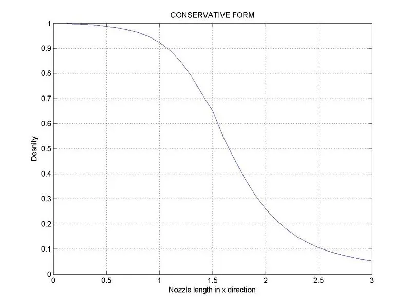
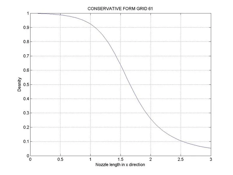
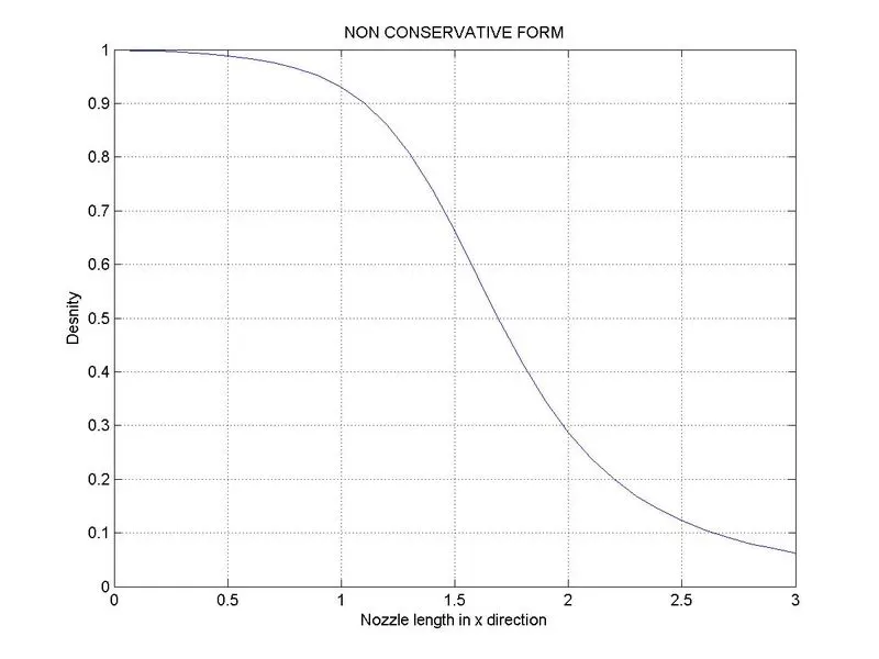
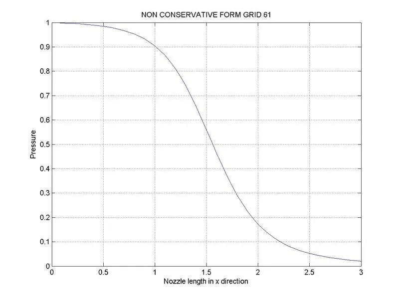
Steady-state distribution of primitive variables inside the nozzle:

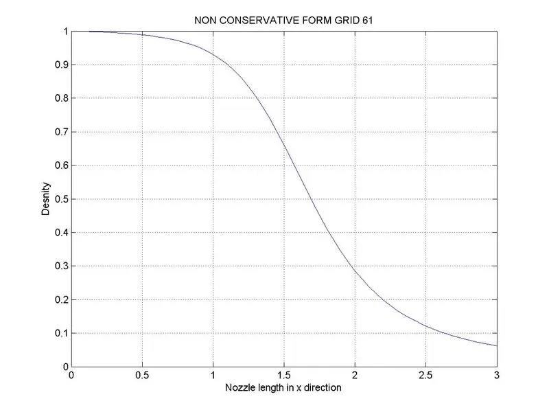
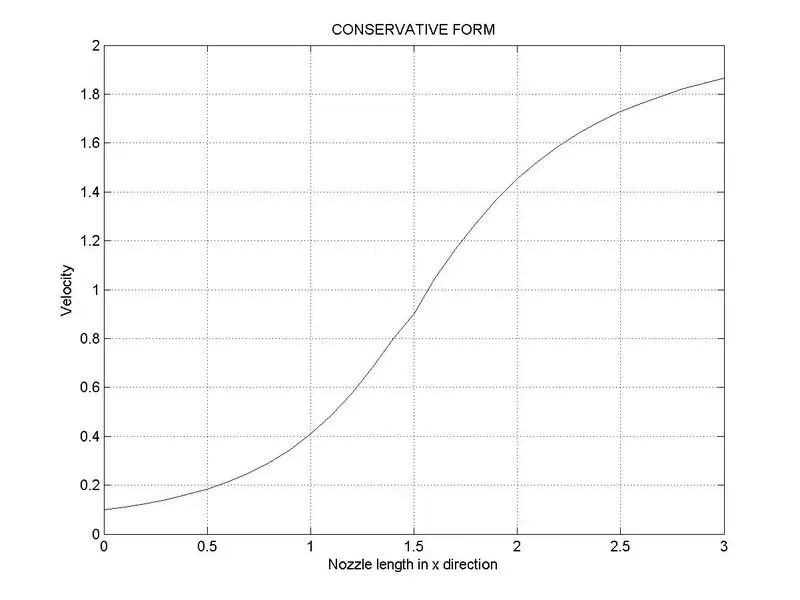
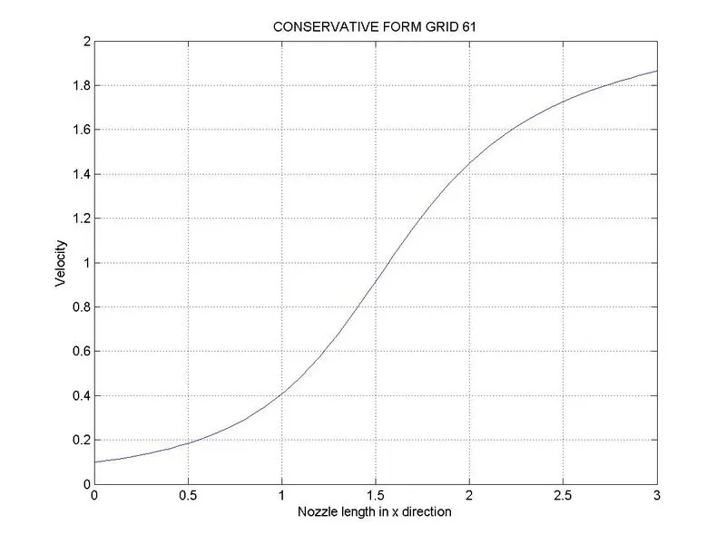
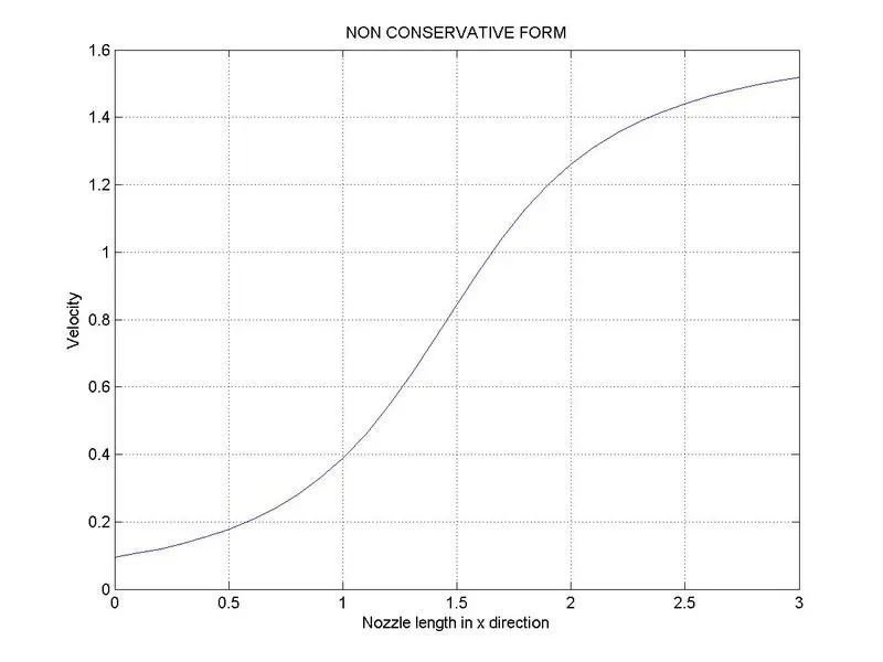
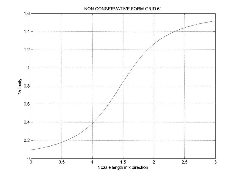
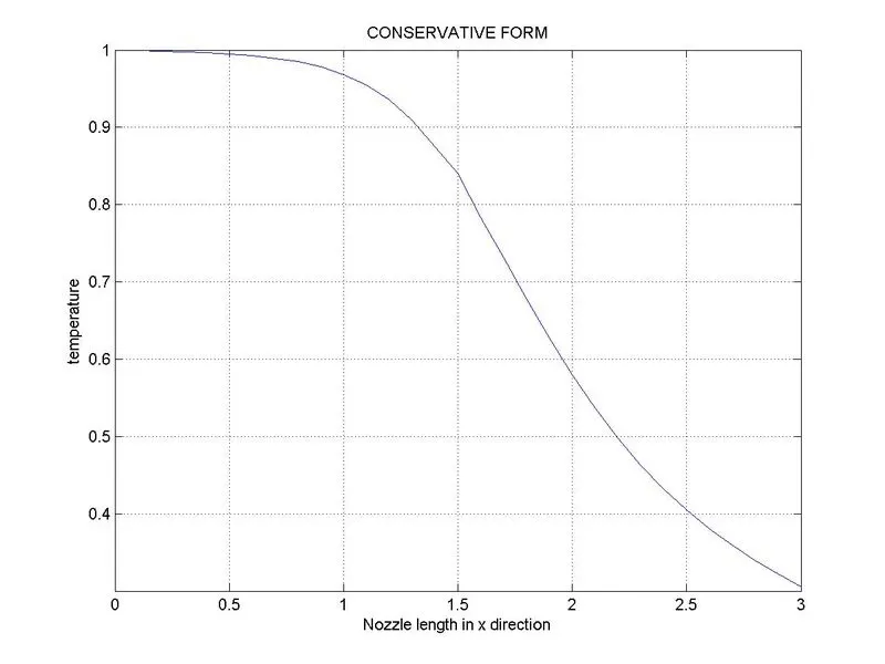
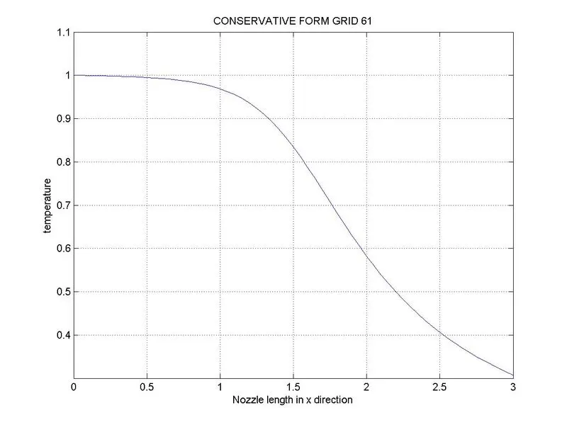
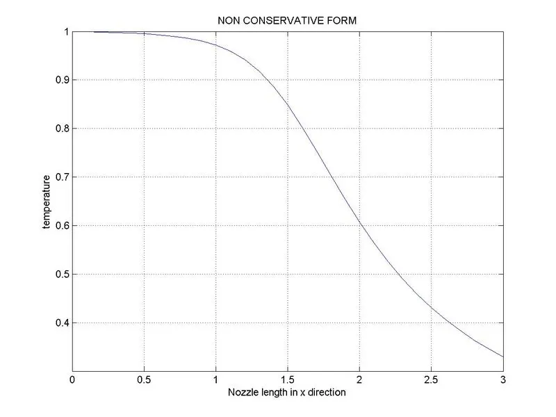
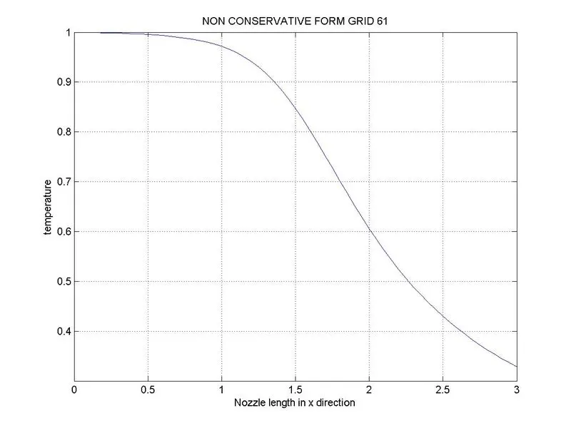
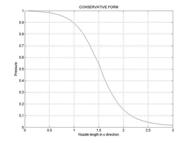
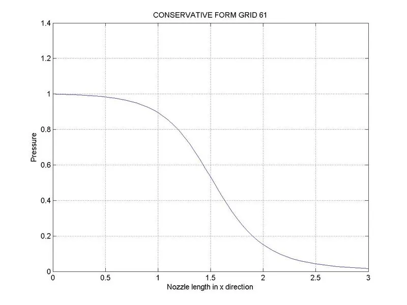
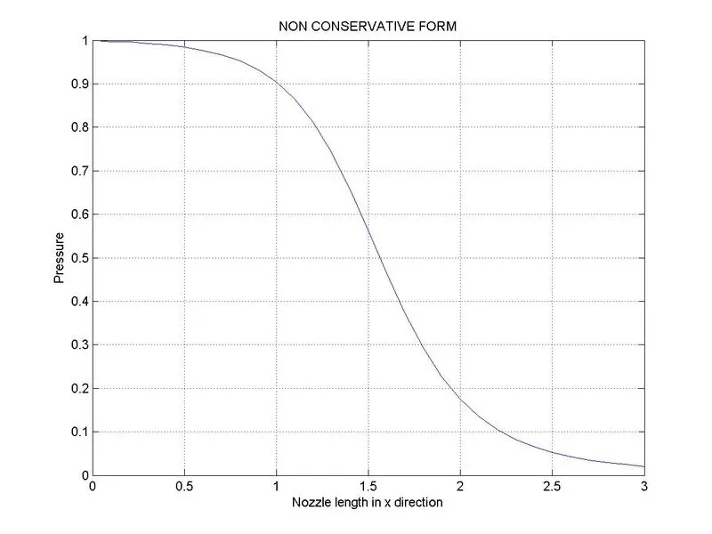
• The graphs are showing the steady-state distribution of density, velocity, temperature, and pressure along the nozzle length in x directions.
• Obtained graphs are in good agreement with the analytical solution to the same problem.
• In both conservative and non-conservative, there is no variation in density and pressure.
• Value of velocity at the outlet is slightly high in conservative form solution than non-conservative form solution (but variations are negligible).
• The value of temperature at the outlet is almost zero in conservative form solution and non-zero in non-conservative form solution(but variations are negligible)..
• Grid wise also, there is very negligible fluctuation in the flow variables value, Hence the obtained solution is grid-independent.

1.Density

Conservative: Grid 31	Conservative: Grid 61	Non-Conservative: Grid 31	Non-Conservative: Grid 61

2.Velocity

Conservative: Grid 31	Conservative: Grid 61	Non-Conservative: Grid 31	Non-Conservative: Grid 61

3.Temperature

Conservative: Grid 31	Conservative: Grid 61	Non-Conservative: Grid 31	Non-Conservative: Grid 61

4.Pressure

Conservative: Grid 31	Conservative: Grid 61	Non-Conservative: Grid 31	Non-Conservative: Grid 61

Steady State distribution of Mass flow rate, and Mach Number:

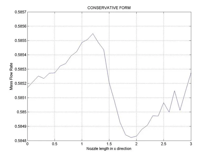
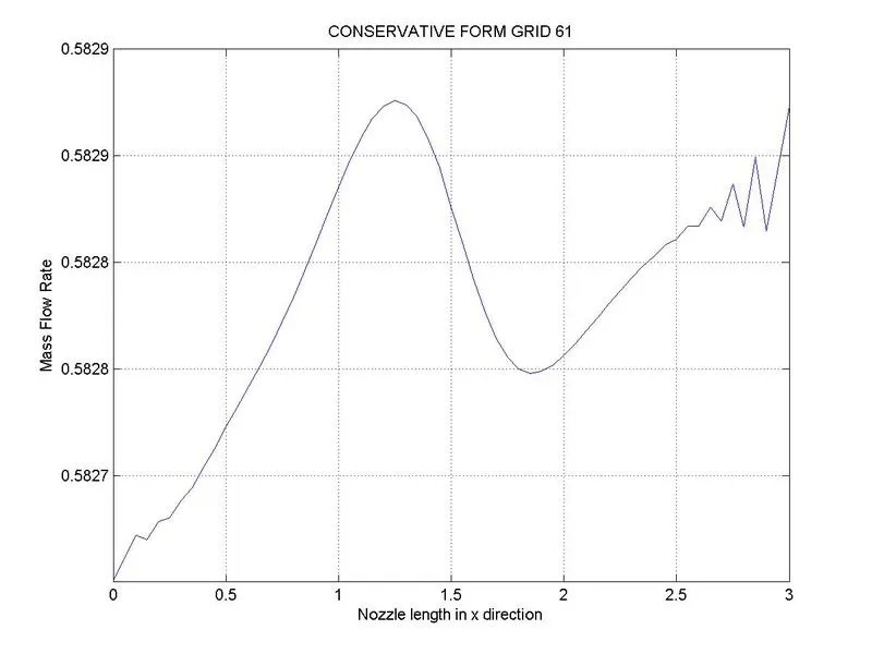
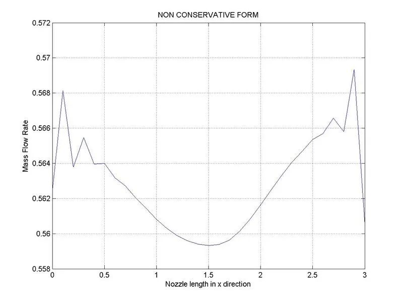
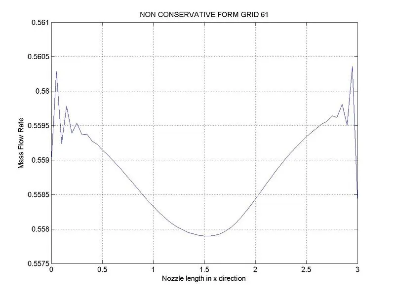
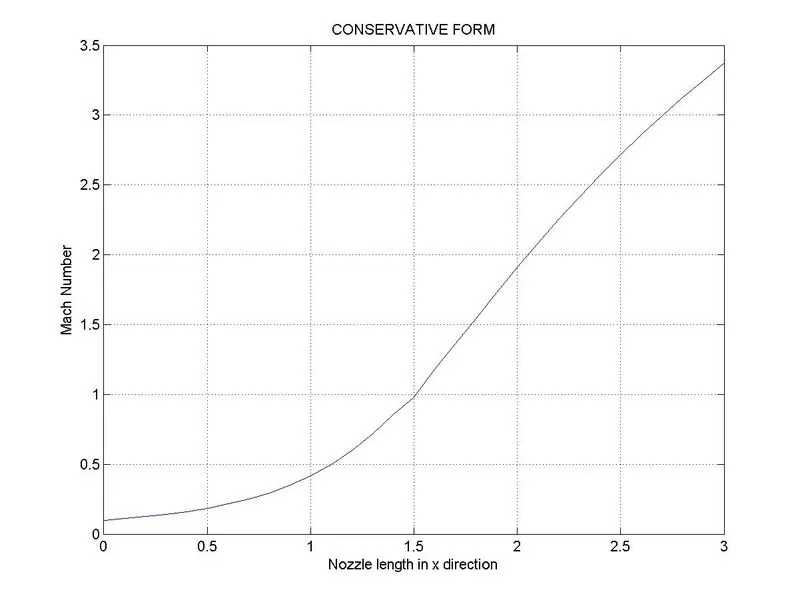
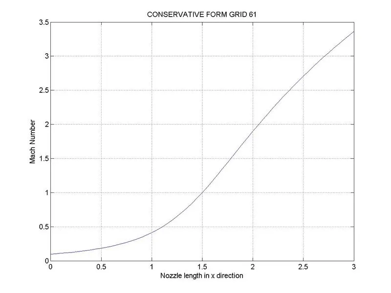
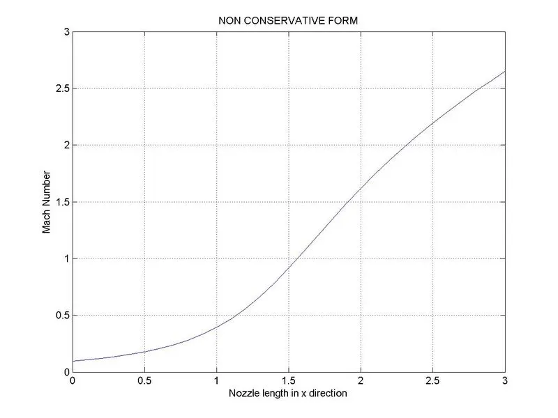
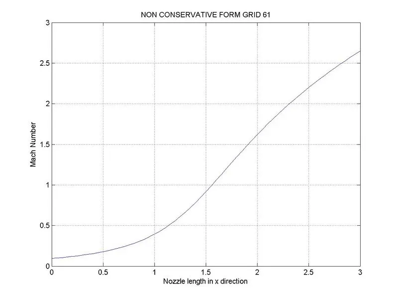
• The graphs are showing the steady-state distribution of Mass flow rate, and Mach number along the nozzle length in x directions.
• Value of mass flow rate becomes almost constant at steady state at the graph showing the fluctuation between values 0.56 to 0.58, it is very negligible.
• At throat value of velocity becomes equal to the local speed of sound, it is captured well by conservative form solution.
• Value of Mach number at the outlet is slightly high in conservative form solution than non-conservative form solution (but variations are negligible).
• Grid wise also, there is very negligible fluctuation in the Mach number value, Hence the obtained solution is grid-independent.
• Similarly, there is very negligible fluctuation in the Mass flow rate value, but at higher grid points curves are smooth comparatively, it is also grid-independent solution.

5.Mass Flow Rate

Conservative: Grid 31	Conservative: Grid 61	Non-Conservative: Grid 31	Non-Conservative: Grid 61

6.Mach Number

Conservative: Grid 31	Conservative: Grid 61	Non-Conservative: Grid 31	Non-Conservative: Grid 61

Time-wise variation of the Flow variables:

• Time-wise variations are captured at each time loop and video is made to see the variation.
• In conservative form, there is a slight fluctuation in mass flow rate is observed even after a steady state is reached.
• Whereas in, non-conservative form, there is no fluctuation in any flow variable, after a steady state is reached.

Conservative: Grid 31	Non-Conservative: Grid 31

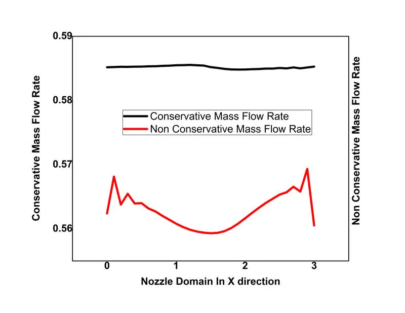
Comparison of Normalized mass flow rate distributions of both forms :

• The conservative form gives a distribution that is much closer to being a constant. in contrast, the nonconservative results have sizeable variation.
• The mass flow rate of conservation form much closer to the exact analytical solution (density*area*velocity = 0.579).

Thank you