Week 3.5 - Deriving 4th order approximation of a 2nd order derivative using Taylor Table method

Derive the following 4th order approximations of the second-order derivative

Aim:

• To derive the 4th order approximation for the second-order derivative of a given function using following 3 schemes.

1. central difference
2. skewed right difference
3. skewed left difference schemes.

Theory:

• If ' X ' is a point(node) in space, at which we need to find the value of a physical quantity (represented in derivative form).
• Taylors-table is one of the methods in finite-difference approximation through which we can covert the derivative form into algebraic form, Hence when this algebraic equation solved at node 'X' gives the value of physical quantity.
• The order of approximation physically representing, "how many neighbouring nodes of 'X' influencing the value of the physical quantity at ' X ' ".
• But order number does not represent the number of neighbouring points affecting the value of the physical quantity at node ' X ', it depends on the type of stencil.
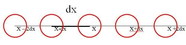
• So stencil is basically a collection of 'neighbouring nodes and node x separated by a distance ' dx ' from one another '. There are two types of stencil, symmetrical stencil and skewed stencil.
• In a symmetrical stencil, the number of neighbouring nodes in the left of node ' X ' is equal to the number of neighbouring nodes in the right of node ' X '.
• In a skewed stencil, the number of neighbouring nodes in the left of node ' X ' is not equal to the number of neighbouring nodes in the right of node ' X '.
• In the left-skewed stencil, all the neighbouring nodes in the stencil present at the left of node 'X' only.
• Similarly in the right-skewed stencil, all the neighbouring nodes in the stencil present at the right of node 'X' only.
• According to the order of approximation, the number of nodes on the stencil changes, it's formula is shown in the below table

For symmetrical stensil	Number of nodes = order of derivative + order of approximation - 1
For skewed stensik	Number of nodes = order of derivative + order of approximation

Working:

• MATLAB is used for coding to achieve the above-mentioned objective.

Given function	exp(x)cos(x)
Second-order Derivative of a function	-2*exp(x)*sin(x)
Order of approximation	4th order approximation
At a Node	X = pi/3 (assumed for problem solving)

1. Central difference

• For central difference, 4th order approximation of second-order derivative,
• number of nodes = 2+4-1 = 5 nodes, Therefore 2 nodes on both side of x.
• It is mathematically represented by

`frac{del^2f}{dx^2}= af(x-2dx)+bf(x-dx)+cf(x)+df(x+dx)+ef(x+2dx)`

	f(x)	dx f'(x)	dx^2 f''(x)	dx^3 f'''(x)	dx^4 f""(x)	dx^5 f""'(x)
a f(x-2dx)	a	-2a	2a	-8a/6	16a/24	-32a/120
b f(x-dx)	b	-b	b/2	-b/6	b/24	-b/120
c f(x)	c	0	0	0	0	0
d f(x+dx)	d	d	d/2	d/6	d/24	d/120
e f(x+2dx)	e	2e	2e	8e/6	16/24	32e/120
	0	0	1	0	0

• equating the first five columns we get five equations, from that we get the values of coefficients" a,b,c,d, and e'

2. Skewed right-sided difference

• For right-skewed difference, 4th order approximation of second-order derivative,
• number of nodes = 2+4 = 6 nodes, Therefore 5 nodes on right side of x.
• It is mathematically represented by

`frac{del^2f}{dx^2}= af(x)+bf(x+dx)+cf(x+2dx)+df(x+3dx)+ef(x+4dx)+gf(x+5dx)`

	f(x)	dx f'(x)	dx^2 f''(x)	dx^3 f'''(x)	dx^4 f""(x)	dx^5 f""'(x)
a f(x)	a	0	0	0	0	0
b f(x+dx)	b	b	b/2	b/6	b/24	b/120
c f(x+2dx)	c	2c	2c	8c/6	16c/24	32c/120
d f(x+3dx)	d	3d	9d/2	27d/6	81d/24	243d/120
e f(x+4dx)	e	4e	16e	64e/6	256/24	1024e/120
g f(x+5dx)	g	5g	25g/2	125g/6	625g/24	3125g/120
	0	0	1	0	0	0

• Equating the first 6 columns we get six equations, from that we get the values of coefficients" a,b,c,d,e and g'

3. Skewed left-sided difference

• For left-skewed difference, 4th order approximation of second-order derivative,
• number of nodes = 2+4 = 6 nodes, Therefore 5 nodes on left side of x.
• It is mathematically represented by

`frac{del^2f}{dx^2}= af(x)+bf(x-dx)+cf(x-2dx)+df(x-3dx)+ef(x-4dx)+gf(x-5dx)`

	f(x)	dx f'(x)	dx^2 f''(x)	dx^3 f'''(x)	dx^4 f""(x)	dx^5 f""'(x)
a f(x)	a	0	0	0	0	0
b f(x-dx)	b	-b	b/2	-b/6	b/24	-b/120
c f(x-2dx)	c	-2c	2c	-8c/6	16c/24	-32c/120
d f(x-3dx)	d	-3d	9d/2	-27d/6	81d/24	-243d/120
e f(x-4dx)	e	-4e	16e	-64e/6	256/24	-1024e/120
g f(x-5dx)	g	-5g	25g/2	-125g/6	625g/24	-3125g/120
	0	0	1	0	0	0

• Equating the first six columns we get six equations, from that we get the values of coefficients" a,b,c,d,e and g'

Code

• In the first step, the x value, second-order derivative of a function at x, Coefficients obtained for different schemes from Taylors tables are defined.
• Range of Discretization Length dx is defined
• For loop is used to find the error value for all the three schemes,at all values of dx
• Relations are established between the variables to solve the fourth-order approximations
• log-log plot is used to compare the error values obtained from a different scheme over a range of 'dx'

clear all
close all
clc 

% to calculate a value of a function at a point x  =pi/3
x= pi/3;

% coeffecient matrix derived for 4th order approximation
% a,b,c,d,e,f,g respectively
% calculated separately

% f''(x) = af(x-2dx)+bf(x-dx)+cf(x)+df(x+dx)+ef(x+2dx)/dx^2
central_scheme = [-0 + 1/(-12);1 + 1/(3);-3 + 1/(2);1 + 1/(3);-0 + 1/(-12)];

% f''(x) = af(x)+bf(x+dx)+cf(x+2dx)+df(x+3dx)+ef(x+4dx)+gf(x+5dx)/dx^2
right_skewed_scheme = [4 + 1/(-4);-13 + 1/(6);18 + 1/(-6);-13;5 + 1/(12);-1 + 1/(6)];

% f''(x) = af(x)+bf(x-dx)+cf(x-2dx)+df(x-3dx)+ef(x-4dx)+gf(x-5dx)/dx^2
left_skewed_scheme = [4 + 1/(-4);-13 + 1/(6);18 + 1/(-6);-13;5 + 1/(12);-1 + 1/(6)];

%given function =exp(x)*cos(x)
%second order derivative of this term
fun_x = exp(x)*cos(x);
second_order_derivative = -2*exp(x)*sin(x);

%discretization length dx
dx = linspace(pi/30,pi/30000,30);

for i = 1:length(dx)
%function at the node points with increment and decrement of dx
fun_xplusdx = exp(x+dx(i))*cos(x+dx(i));
fun_xplus2dx = exp(x+(2*dx(i)))*cos(x+(2*dx(i)));
fun_xplus3dx = exp(x+(3*dx(i)))*cos(x+(3*dx(i)));
fun_xplus4dx = exp(x+(4*dx(i)))*cos(x+(4*dx(i)));
fun_xplus5dx = exp(x+(5*dx(i)))*cos(x+(5*dx(i)));
fun_xminusdx = exp(x-dx(i))*cos(x-dx(i));
fun_xminus2dx = exp(x-(2*dx(i)))*cos(x-(2*dx(i)));
fun_xminus3dx = exp(x-(3*dx(i)))*cos(x-(3*dx(i)));
fun_xminus4dx = exp(x-(4*dx(i)))*cos(x-(4*dx(i)));
fun_xminus5dx = exp(x-(5*dx(i)))*cos(x-(5*dx(i)));

%cental difference scheme of 4 the order
C_1 = central_scheme(1)*fun_xminus2dx;
C_2 = central_scheme(2)*fun_xminusdx;
C_3 = central_scheme(3)*fun_x;
C_4 = central_scheme(4)*fun_xplusdx;
C_5 = central_scheme(5)*fun_xplus2dx;

central_fourth(i) = (C_1+C_2+C_3+C_4+C_5)/(dx(i)^2);
central_error(i) = abs(central_fourth(i)-second_order_derivative);

%for right skewed scheme of 4th order approximation
R_1 = right_skewed_scheme(1)*fun_x;
R_2 = right_skewed_scheme(2)*fun_xplusdx;
R_3 = right_skewed_scheme(3)*fun_xplus2dx;
R_4 = right_skewed_scheme(4)*fun_xplus3dx;
R_5 = right_skewed_scheme(5)*fun_xplus4dx;
R_6 = right_skewed_scheme(6)*fun_xplus5dx;

R_skewed_fourth(i) = (R_1+R_2+R_3+R_4+R_5+R_6)/(dx(i)^2);
Rskewed_error(i) = abs(R_skewed_fourth(i)-second_order_derivative);

%for left skewed scheme of 4th order approximation
L_1 = left_skewed_scheme(1)*fun_x;
L_2 = left_skewed_scheme(2)*fun_xminusdx;
L_3 = left_skewed_scheme(3)*fun_xminus2dx;
L_4 = left_skewed_scheme(4)*fun_xminus3dx;
L_5 = left_skewed_scheme(5)*fun_xminus4dx;
L_6 = left_skewed_scheme(6)*fun_xminus5dx;

L_skewed_fourth(i) = (L_1+L_2+L_3+L_4+L_5+L_6)/(dx(i)^2);
Lskewed_error(i) =  abs(L_skewed_fourth(i)-second_order_derivative);

end

figure(1)
loglog(dx,central_error,'linewidth',3,'color','r')
hold on
loglog(dx,Rskewed_error,'linewidth',3,'color','b')
hold on
loglog(dx,Lskewed_error,'linewidth',3,'color','g')
legend('central scheme error','right skewed scheme error','left skewed schee error')
xlabel('range of dx')
ylabel('Truncation error')
title('Comparision of central, right skewed and left skewed 4th order approximation for second order derivative')

Result:

• The code ran successfully.
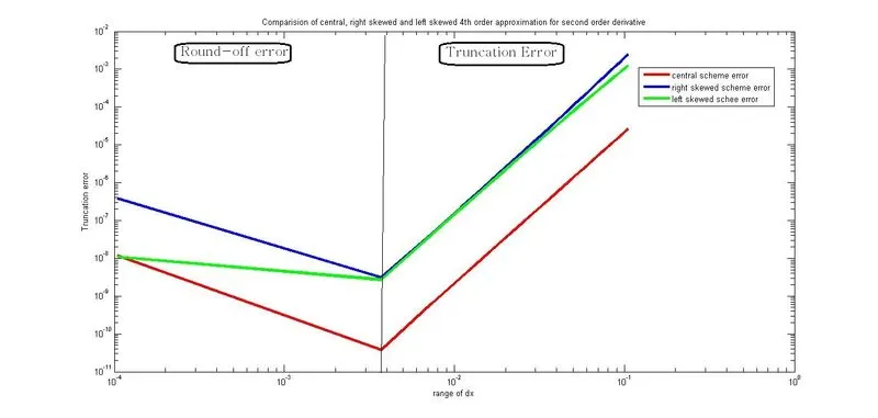
• From the result, it can be seen that central difference scheme error values are less compared to skewed difference scheme error values.
• As the value of dx decreases, the truncation error value also decreases.
• Due to the computer storage capacity, roundoff error is observed after a certain value of dx, it is indicated by the region representing increasing error values with a decrease in dx.

Thank you