Week 9 - FVM Literature Review

FINITE VOLUME METHOD

Definition: It is one of the numerical technique employed by CFD to solve the governing equations which govern the fluid flow phenomenon and other fluid flow-associated phenomenon, by defining the value of the flow variables at the centroid of the control volume.

Theory:

• Governing equations are obtained either in integral form and differential form.
• These governing equations represent the values of flow variables at each and every point in the flow domain( continuous function).
• Discretization is a process of converting differential or integral equations of governing equations into algebraic equations.
• These algebraic equations approximate the value of flow variables only at a finite number of discrete points in the flow domain (not continuous).
• Finite Difference Method, Finite Volume Method, and Finite Element Method are the discretization techniques used by CFD.

Finite Volume Method	Finite Difference Method
It uses an integral form of governing equation to discretize the flow domain	It uses a differential form of governing equations to discretize the flow domain
It stores the flow variable values at the centroid of the control volume	It stores the flow variable value at the mesh grid points.
Its mathematical expression represents the conservation of the fluid property.	Its mathematical expression does not represent the conservation of the fluid property
It can be used easily, even when grids are not aligned(Unstructured mesh)	It cannot be used easily when grids are not aligned (transformation functions are required)

FVM Steps:

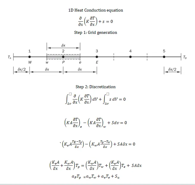
Step 1: Grid generation

• The first step of the FVM is to divide the domain into discrete control volumes.
• The boundaries (or faces) of control volumes are positioned mid-way between adjacent nodes.

Step 2: Discretisation

• The key step of the finite volume method is the integration of the governing equations over a control volume to yield a discretized equation at its centroid.

Step 3: Solution of equations

• Discretised equations set up at each of the nodal points.
• For control volumes that are adjacent to the domain boundaries the discretized equation must be modified to incorporate boundary conditions.
• The resulting system of linear algebraic equations is then solved using a suitable matrix method to obtain the distribution of the flow properties at nodal points.

1D linear heat conduction equation

• It is a steady-state pure diffusion process.
• FVM Steps are explained in the below figure

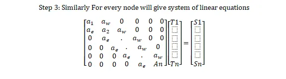
• The above-obtained system of linear equations is solved using a suitable matrix method.
• In order to derive useful forms of the discretised equations, the interface diffusion coefficient K and the gradient dT/dx at the east and west are required.
• But the values of the property T and the diffusion coefficient are defined and evaluated at nodal points(centroid).
• To calculate gradients dT/dx (and hence fluxes) at the control volume faces an approximate distribution of properties between nodal points is used, i.e Gradient Scheme.
• To calculate diffusive terms at the control faces, Interpolation schemes are used to transform cell-centre quantities to face centres.

Note: In OpenFOAM

• Flux limiters are used to preserve the monotonicity condition by limiting the flux to ensure that the extrapolated flux value at faces is bounded by the neighbouring cell values.

Thank You