Week 12 - Validation studies of Symmetry BC vs Wedge BC in OpenFOAM vs Analytical H.P equation
Validation studies of Symmetry BC vs Wedge BC in OpenFOAM vs Analytical H.P equation
AIM:
- To simulate flow through pipe in OpenFOAM, using symmetry boundary condition and wedge boundary condition separately.
- To compare the simulation result with Hagen–Poiseuille fully developed flow equation.
THEORY:
- Haigen-Poiseuille flow is defined for steady state incompressible fully developed laminar flow in a horizontal pipe/duct.
- Velocity fully developed means, axial velocity does not varies in the flow direction, it remains constant.
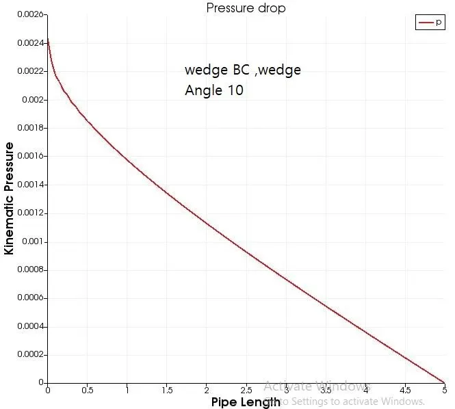
- Axial velocity u (velocity along flow direction) is positive along the radial direction and it varies parabolically along the radial direction, and thus the axial pressure gradient dP/dx must be negative,i.e., pressure must decrease in the flow direction because of viscous effects—it takes pressure to push the fluid through the pipe.
- The average velocity in fully developed laminar pipe flow is one half of the maximum velocity(present at the center of the pipe low)
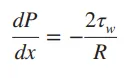
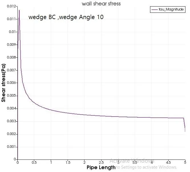
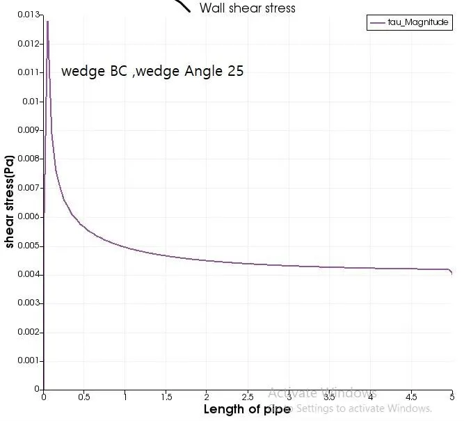
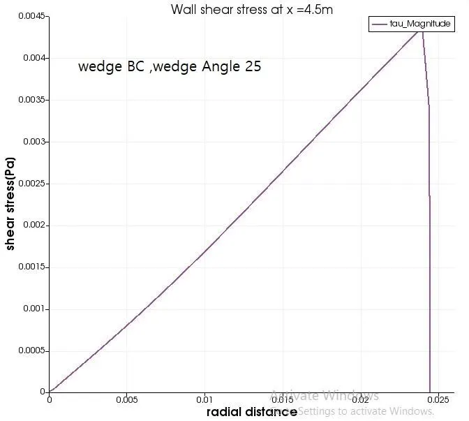
- The shear stress at the pipe wall is related to the slope of the velocity profile at the surface. Noting that the velocity profile remains unchanged in the hydrodynamically fully developed region, the wall shear stress also remains constant in that region.
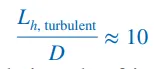
- To find the length of entrance effect is given by
- To find the pressure drop variation with shear stress along the length of the pipe or vice-versa.
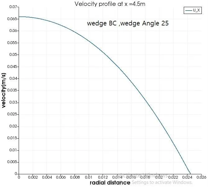
- To find the variation of axial velocity in radial direction in the fully developed region is given by
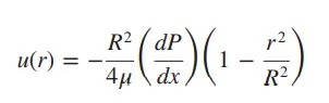 NOTE: at center(r=0) and at the wall(r=R)
- Relation Between Mean and maximum velocity.
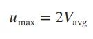
- This relations are Haigen posruille relations valid only only in fully developed region.
- Using above relations simulation results are validated.
OpenFOAM:
- Workflow is similar to previous challenge.
- Water is selected as working fluid with density = 995.6kg/m^3 and viscosity = 0.0007972 Ns/m^2 at 30 degree celsius
- Here wedge angle 10,25 and 45 degree is considered for generation of axis-symmetric section.
- And each geometries are again simulated for 2 different patch type.
- one is symmetric patch type and second one is wedge patch type for front and back wall of geometry.
- icoFoam is the solver used to simulate the transient laminar viscous flow in the OpenFOAM
- In the icoFoam system folder, the blockMeshDict file is used to generate the flow geometry and mesh.
- The diameter is assumed as 5cm and according to the given Reynold number at the inlet(2100), boundary condition velocity at inlet is calculated in meters.
- Length is assumed by keeping the hydrodynamic entrance length relation in mind.
- According to the velocity, simulation time and time steps are defined in the controlDict file.
- Inlet velocity and outlet pressure values are defined in the P & U files present in the 0 folders.
- In transportproperties folder, the kinematic viscosity of water at 30 degrees celsius is defined.
- Since wedge boundary condition is simulated in previous challenge, Here i am showing code files belongs to symmetric boundary conditions only.
- Note: For different wedge angle, changes are done only in the blockMeshDict file, remaining files remains same.
blockMeshDict: wedge angle(45 degree)
/*--------------------------------*- C++ -*----------------------------------*\
  =========                 |
  \\      /  F ield         | OpenFOAM: The Open Source CFD Toolbox
   \\    /   O peration     | Website:  https://openfoam.org
    \\  /    A nd           | Version:  8
     \\/     M anipulation  |
\*---------------------------------------------------------------------------*/
FoamFile
{
    version     2.0;
    format      ascii;
    class       dictionary;
    object      blockMeshDict;
}
// * * * * * * * * * * * * * * * * * * * * * * * * * * * * * * * * * * * * * //

convertToMeters 0.01;

vertices
(
     (0.0000 0.0000 0.0000 )
     (500.0000 0.0000 0.0000 )
     (500.0000 2.3097 0.9567 )
     (0.0000 2.3097 0.9567 )
     (500.0000 2.3097 -0.9567 )
     (0.0000 2.3097 -0.9567 )
);

blocks
(
    hex (0 5 3 0 1 4 2 1) (100 1 100) simpleGrading (1 1 1)
);

edges
(
);

boundary
(
    axis
    {
        type empty;
        faces
        (
            (0 1 1 0)
        );
    }
    inlet
    {
        type patch;
        faces
        (
            (0 3 5 0)
        );
    }
    outlet
    {
        type patch;
        faces
        (
            (1 4 2 1)
        );
    }
    noslipwalls
    {
        type wall;
        faces
        (
            (3 2 4 5)
        );
    }
    front
    {
        type symmetry;
        faces
        (
            (0 1 2 3)
        );
    }
    back
    {
        type symmetry;
        faces
        (
            (0 5 4 1)
        );
    }
);
mergePatchPairs
(
);

// *************************************************************************
ControlDict
/*--------------------------------*- C++ -*----------------------------------*\
  =========                 |
  \\      /  F ield         | OpenFOAM: The Open Source CFD Toolbox
   \\    /   O peration     | Website:  https://openfoam.org
    \\  /    A nd           | Version:  8
     \\/     M anipulation  |
\*---------------------------------------------------------------------------*/
FoamFile
{
    version     2.0;
    format      ascii;
    class       dictionary;
    location    "system";
    object      controlDict;
}
// * * * * * * * * * * * * * * * * * * * * * * * * * * * * * * * * * * * * * //

application     icoFoam;

startFrom       startTime;

startTime       0;

stopAt          endTime;

endTime         180;

deltaT          0.05;

writeControl    timeStep;

writeInterval   20;

purgeWrite      0;

writeFormat     ascii;

writePrecision  6;

writeCompression off;

timeFormat      general;

timePrecision   6;

runTimeModifiable true;


// ************************************************************************* //
pressure P
/*--------------------------------*- C++ -*----------------------------------*\
  =========                 |
  \\      /  F ield         | OpenFOAM: The Open Source CFD Toolbox
   \\    /   O peration     | Website:  https://openfoam.org
    \\  /    A nd           | Version:  8
     \\/     M anipulation  |
\*---------------------------------------------------------------------------*/
FoamFile
{
    version     2.0;
    format      ascii;
    class       volScalarField;
    object      p;
}
// * * * * * * * * * * * * * * * * * * * * * * * * * * * * * * * * * * * * * //

dimensions      [0 2 -2 0 0 0 0];

internalField   uniform 0;

boundaryField
{
    axis
    {
        type            empty;
    }

    inlet
    {
        type            zeroGradient;
    }

    outlet
    {
        type            fixedValue;
        value           uniform 0;
    }

    noslipwalls
    {
        type            zeroGradient;
    }

    front
    {
        type            symmetry;
    }

    back
    {
        type            symmetry;
    }
}
// ************************************************************************* //
Velocity u
/*--------------------------------*- C++ -*----------------------------------*\
  =========                 |
  \\      /  F ield         | OpenFOAM: The Open Source CFD Toolbox
   \\    /   O peration     | Website:  https://openfoam.org
    \\  /    A nd           | Version:  8
     \\/     M anipulation  |
\*---------------------------------------------------------------------------*/
FoamFile
{
    version     2.0;
    format      ascii;
    class       volVectorField;
    object      U;
}
// * * * * * * * * * * * * * * * * * * * * * * * * * * * * * * * * * * * * * //

dimensions      [0 1 -1 0 0 0 0];

internalField   uniform (0 0 0);

boundaryField
{
    axis
    {
        type            empty;
    }

    inlet
    {
        type            fixedValue;
        value           uniform (0.0336294 0 0);
    }

    outlet
    {
        type            zeroGradient;
    }

    noslipwalls
    {
        type            noSlip;
    }

    front
    {
        type            symmetry;
    }

    back
    {
        type            symmetry;
    }
}

// ************************************************************************* //
Kinematic viscosity transport properties
/*--------------------------------*- C++ -*----------------------------------*\
  =========                 |
  \\      /  F ield         | OpenFOAM: The Open Source CFD Toolbox
   \\    /   O peration     | Website:  https://openfoam.org
    \\  /    A nd           | Version:  8
     \\/     M anipulation  |
\*---------------------------------------------------------------------------*/
FoamFile
{
    version     2.0;
    format      ascii;
    class       dictionary;
    location    "constant";
    object      transportProperties;
}
// * * * * * * * * * * * * * * * * * * * * * * * * * * * * * * * * * * * * * //

nu              [0 2 -1 0 0 0 0] 0.0000008007;


// ************************************************************************* //
RESULT:
10 degree
| Symmetric Boundary Condition | Wedge Boundary Condition | |
| Graph1 | 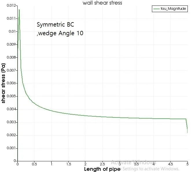 |
 |
| Graph2 | 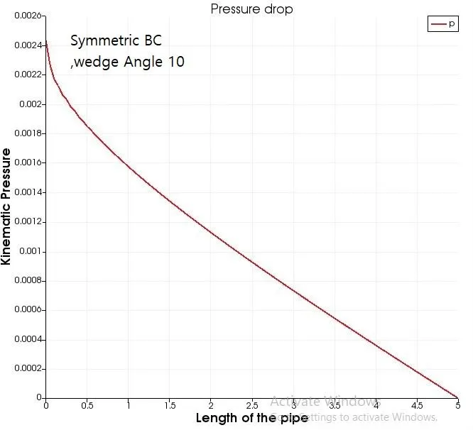 |
 |
| Graph3 | 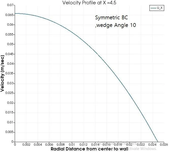 |
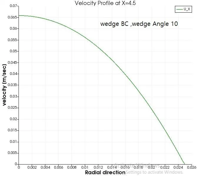 |
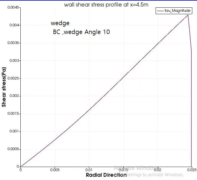
| Graph4 | 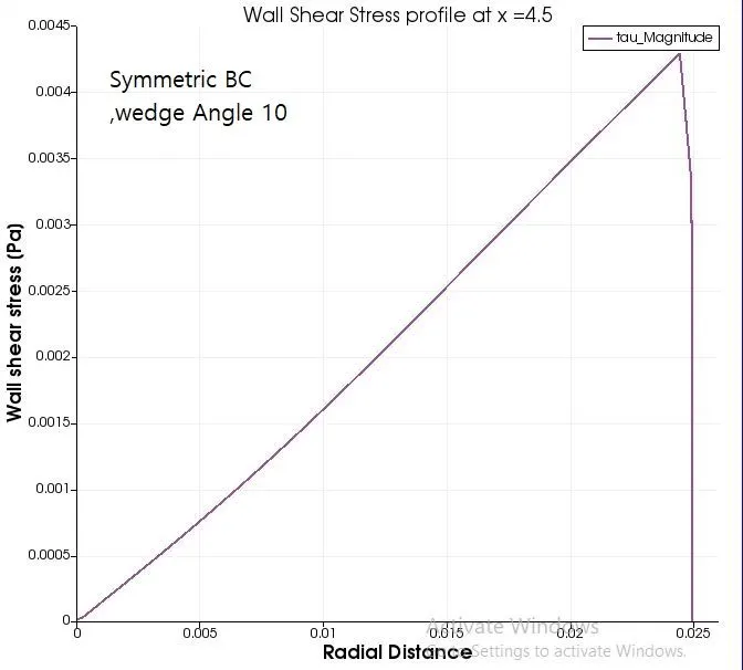 |
 |
| Validation of Hydro-dynamic length with the wall shear stress graph |
|
|
| Validation of fully developed flow velocity profile with its analytical profile and Validation of maximum velocity and pressure drop for fully developed flow |
|
|
| validation of wall shear stress for fully developed flow |
|
|
25 degree
| Symmetric Boundary Condition | Wedge Boundary Condition | |
| Graph5 | 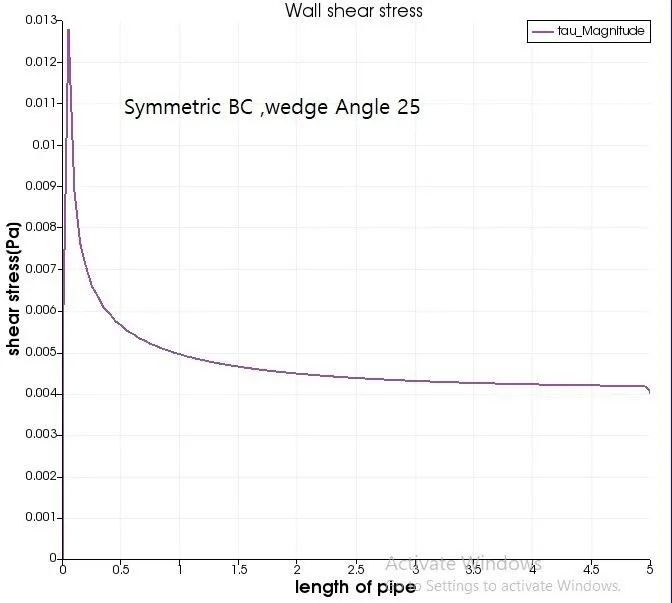 |
 |
| Graph6 | 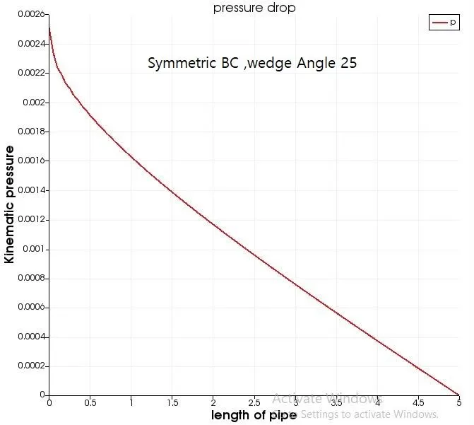 |
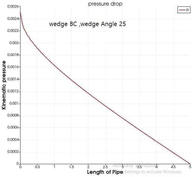 |
| Graph7 | 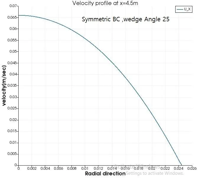 |
 |
| Graph8 | 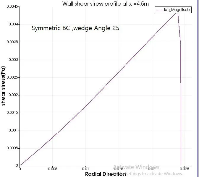 |
 |
| Validation of Hydro-dynamic length with the wall shear stress graph |
|
|
| Validation of fully developed flow velocity profile with its analytical profile and Validation of maximum velocity and pressure drop for fully developed flow |
|
|
| validation of wall shear stress for fully developed flow |
|
|
45 degree
| Symmetric Boundary Condition | Wedge Boundary Condition | |
| Graph9 | 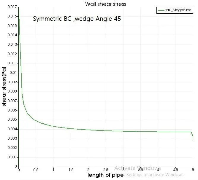 |
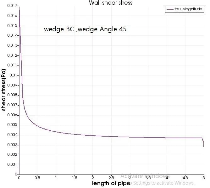 |
| Graph10 | 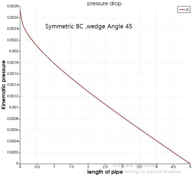 |
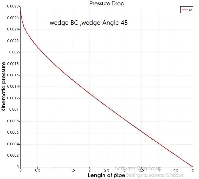 |
| Graph11 | 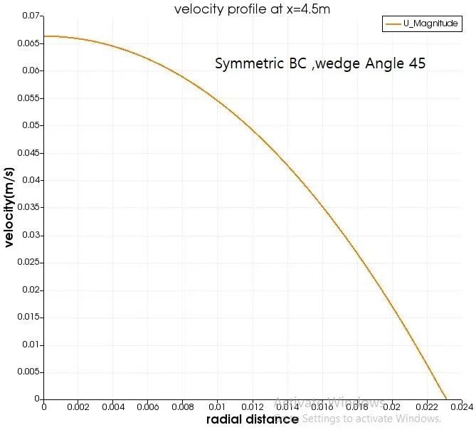 |
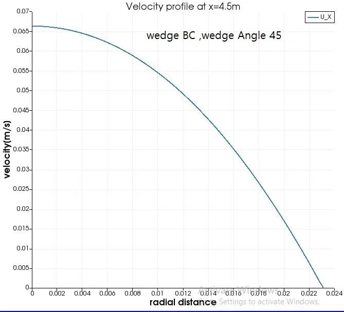 |
| Graph12 | 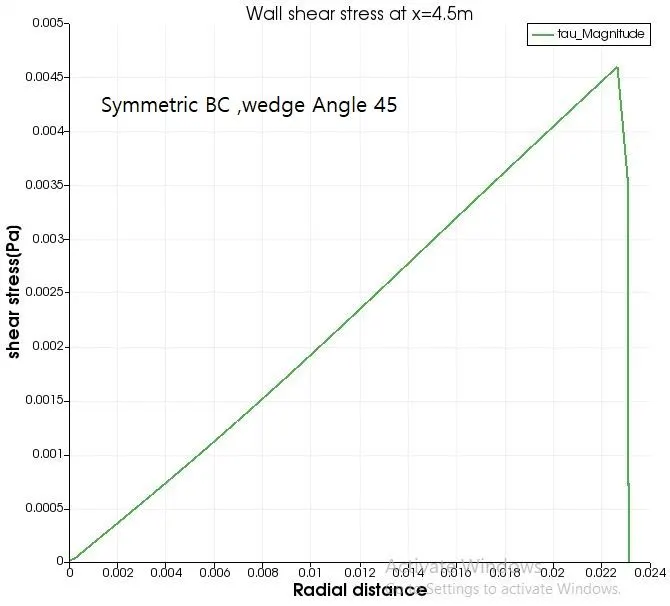 |
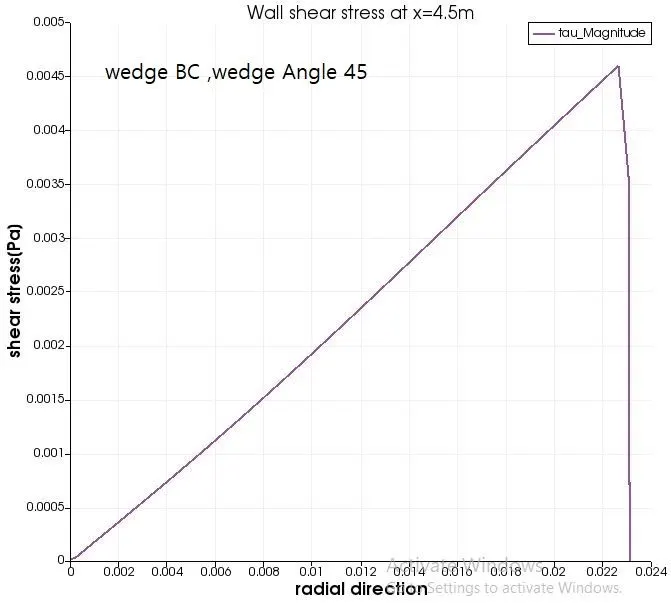 |
| Validation of Hydro-dynamic length with the wall shear stress graph |
|
|
| Validation of fully developed flow velocity profile with its analytical profile and Validation of maximum velocity and pressure drop for fully developed flow |
|
|
| validation of wall shear stress for fully developed flow |
|
|
Conclusion:
- No major variation in simulation result is observed at wedge angle 10 and 25 degree, but at wedge angle 45 degree simulation result shows variation.
- Simulation At wedge angle 45, the error between simulation result and theoretical result is increased.
- For both the wedge and symmetry boundary conditions simulation giving same result.
- Symmetry boundary conditions, mirrors the geometry about the front and back faces.
- Where as wedge boundary conditions, does the same about axis of symmetry.
Thankyou