Week 11 - Simulation of Flow through a pipe in OpenFoam
Simulation of Flow through a pipe in OpenFoam
AIM:
To carry out transient simulation of fully developed laminar flow through the pipe using OpenFOAM and validation of simulation results with the Hagen- Poiseuille's equations for the fully developed flow.
THEORY:
Internal Flow and significance of Reynolds Number
- Fluid flow is classified into two types internal flow and external flow, Internal flow is the one where duct/pipe is completely filled by fluid and the flow is driven primarily by pressure difference.
- In general, flow sections of the circular cross-section are referred to as pipes and flow sections of non-circular cross-section as ducts. Small diameter pipes are usually referred to as tubes. Generally, pipes withstand large pressure differences between inside and outside of the pipe, without significant distortion, and hence, especially liquids are transported in circular pipes.
- In internal flow, fluid flow further divided into laminar and turbulent flow.
- Laminar flow, characterized by the assumption that fluid composed of layers, and the highly ordered motion of these layers constitutes the laminar flow.
- Turbulent flow is characterized by the inter-mixing of fluid layers, velocity fluctuations, and highly disordered motion.
- Reynolds number is a dimensionless number, it is a ratio of inertial forces to viscous forces in the fluid. This ratio defines whether the flow is laminar or turbulent.

- In laminar flow, Reynolds number shows a small value,i.e, the viscous forces are large enough to suppress inertial forces to keep the fluid layers intact.
- In turbulent flow, Reynolds number shows a large value,i.e, the viscous forces are not large enough to suppress inertial forces to keep the fluid layers intact, resulting in intermixing of fluid layers, resulting in momentum transfer between the fluid particles, therefore increase in friction force causes the massive pressure drop.
- For internal flow in a circular pipe, the generally accepted value of the critical Reynolds number is 2300, below which flow is laminar and above which flow is turbulent.
Laminar flow in a pipe
- At the entry of the fluid into the pipe, due to the no-slip boundary condition at the wall, the fluid particles in the layer in contact with the wall come to a complete stop.it also causes the fluid particles in the adjacent layers to slow down gradually as a result of friction force(viscous force). To make up for this velocity reduction, the velocity of the fluid at the midsection of the pipe has to increase to keep the mass flow rate through the pipe constant. As a result, a velocity gradient develops along the pipe, it creates a hypothetical boundary surface called the boundary layer region.
- Therefore hypothetical boundary surface is created and divides the flow in a pipe into two regions: the boundary layer region, in which the viscous effects and the velocity changes are significant, and the free stream flow (irrotational) flow region, in which the frictional effects are negligible and the velocity remains essentially constant in the radial direction.
- At the starting of the inlet thickness of the boundary-layer region is zero and thickness starts to increase in the flow direction until the boundary layer reaches the pipe center and thus fills the entire pipe, and the velocity becomes fully developed.
- The region from the pipe inlet, to the point at which the velocity profile is fully developed, is called the hydrodynamic entrance region.
- The region beyond the hydrodynamic entrance region in which the velocity profile is fully developed and remains unchanged is called the hydrodynamically fully developed region.
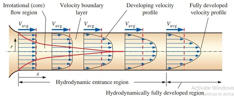
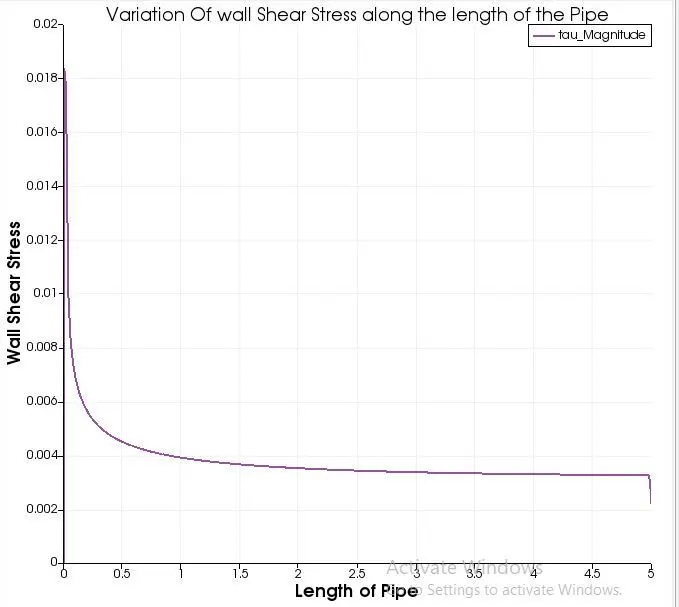
- The wall shear stress is the highest at the pipe inlet where the thickness of the boundary layer is smallest and decreases gradually with an increase in boundary layer thickness until its value equals the wall shear stress at the fully developed region. Therefore, the pressure drop is higher in the entrance regions of a pipe.
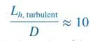
- In many pipe flows of practical engineering interest, the entrance effects become insignificant beyond a pipe length equals to 10 times the pipe diameter.
- It is given by
Fully Developed Laminar flow through the pipe
- It is also called Hagen–Poiseuille flow, it is defined by assuming fluid is incompressible, flow is steady, fluid flows in a horizontal pipe, 1D flow, and velocity is developed.
- Velocity fully developed means, axial velocity does not varies in the flow direction, it remains constant.
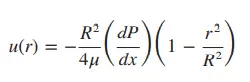
- Axial velocity u (velocity along flow direction) is positive along the radial direction and it varies parabolically along the radial direction, and thus the axial pressure gradient dP/dx must be negative,i.e., pressure must decrease in the flow direction because of viscous effects—it takes pressure to push the fluid through the pipe.
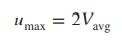
- The average velocity in fully developed laminar pipe flow is one half of the maximum velocity(present at the center of the pipe low)
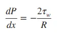
- The shear stress at the pipe wall is related to the slope of the velocity profile at the surface. Noting that the velocity profile remains unchanged in the hydrodynamically fully developed region, the wall shear stress also remains constant in that region.
 ,
,  ,
,
- Above relations are valid for Fully developed Laminar flow region only.
OpenFOAM:
- Water is selected as working fluid with density = 995.6kg/m^3 and viscosity = 0.0007972 Ns/m^2 at 30 degree celsius.
- icoFoam is the solver used to simulate the transient laminar viscous flow in the OpenFOAM
- In the icoFoam system folder, the blockMeshDict file is used to generate the flow geometry and mesh.
- To make the simulation smoother, only the wedge section of the pipe is defined along the axis of symmetry.
- The wedge section is also called the axis-symmetric section with a wedge angle less than 5 degrees. It is created by collapsing the two vertices of the hexagonal block.
- Here the walls of the axis-symmetric section are indicated by a patch type called "Wedge".
- The diameter is assumed as 5cm and according to the given Reynold number at the inlet(2100), boundary condition velocity at inlet is calculated in meters.
- Length is assumed by keeping the hydrodynamic entrance length relation in mind.
- According to the velocity, simulation time and time steps are defined in the controlDict file.
- Inlet velocity and outlet pressure values are defined in the P & U files present in the 0 folders.
- In transportproperties folder, the kinematic viscosity of water at 30 degrees celsius is defined.
system folder:blockMeshDict
/*--------------------------------*- C++ -*----------------------------------*\
  =========                 |
  \\      /  F ield         | OpenFOAM: The Open Source CFD Toolbox
   \\    /   O peration     | Website:  https://openfoam.org
    \\  /    A nd           | Version:  8
     \\/     M anipulation  |
\*---------------------------------------------------------------------------*/
FoamFile
{
    version     2.0;
    format      ascii;
    class       dictionary;
    object      blockMeshDict;
}
// * * * * * * * * * * * * * * * * * * * * * * * * * * * * * * * * * * * * * //

convertToMeters 0.01;

vertices
(
    (0 0 0)
    (500 0 0)
    (500 2.4976 0.109048)
    (0 2.4976 0.109048)
    (500 2.4976 -0.109048)
    (0 2.4976 -0.109048)

);

blocks
(
    hex (0 5 3 0 1 4 2 1) (200 1 250) simpleGrading (1 1 1)
);

edges
(
);

boundary
(
    axis
    {
        type empty;
        faces
        (
            (0 1 1 0)
        );
    }
    inlet
    {
        type patch;
        faces
        (
            (0 3 5 0)
        );
    }
    outlet
    {
        type patch;
        faces
        (
            (1 4 2 1)
        );
    }
    noslipwalls
    {
        type wall;
        faces
        (
            (3 2 4 5)
        );
    }
    front
    {
        type wedge;
        faces
        (
            (0 1 2 3)
        );
    }
    back
    {
        type wedge;
        faces
        (
            (0 5 4 1)
        );
    }
);
mergePatchPairs
(
);

// *************************************************************************
system folder:ControlDict
/*--------------------------------*- C++ -*----------------------------------*\
  =========                 |
  \\      /  F ield         | OpenFOAM: The Open Source CFD Toolbox
   \\    /   O peration     | Website:  https://openfoam.org
    \\  /    A nd           | Version:  8
     \\/     M anipulation  |
\*---------------------------------------------------------------------------*/
FoamFile
{
    version     2.0;
    format      ascii;
    class       dictionary;
    location    "system";
    object      controlDict;
}
// * * * * * * * * * * * * * * * * * * * * * * * * * * * * * * * * * * * * * //

application     icoFoam;

startFrom       startTime;

startTime       0;

stopAt          endTime;

endTime         180;

deltaT          0.05;

writeControl    timeStep;

writeInterval   20;

purgeWrite      0;

writeFormat     ascii;

writePrecision  6;

writeCompression off;

timeFormat      general;

timePrecision   6;

runTimeModifiable true;


// ************************************************************************* //
0 folder:Preesure p
/*--------------------------------*- C++ -*----------------------------------*\
  =========                 |
  \\      /  F ield         | OpenFOAM: The Open Source CFD Toolbox
   \\    /   O peration     | Website:  https://openfoam.org
    \\  /    A nd           | Version:  8
     \\/     M anipulation  |
\*---------------------------------------------------------------------------*/
FoamFile
{
    version     2.0;
    format      ascii;
    class       volScalarField;
    object      p;
}
// * * * * * * * * * * * * * * * * * * * * * * * * * * * * * * * * * * * * * //

dimensions      [0 2 -2 0 0 0 0];

internalField   uniform 0;

boundaryField
{
    axis
    {
        type            empty;
    }

    inlet
    {
        type            zeroGradient;
    }

    outlet
    {
        type            fixedValue;
        value           uniform 0;
    }

    noslipwalls
    {
        type            zeroGradient;
    }

    front
    {
        type            wedge;
    }

    back
    {
        type            wedge;
    }
}
// ************************************************************************* //
0 folder:Velocity U
/*--------------------------------*- C++ -*----------------------------------*\
  =========                 |
  \\      /  F ield         | OpenFOAM: The Open Source CFD Toolbox
   \\    /   O peration     | Website:  https://openfoam.org
    \\  /    A nd           | Version:  8
     \\/     M anipulation  |
\*---------------------------------------------------------------------------*/
FoamFile
{
    version     2.0;
    format      ascii;
    class       volVectorField;
    object      U;
}
// * * * * * * * * * * * * * * * * * * * * * * * * * * * * * * * * * * * * * //

dimensions      [0 1 -1 0 0 0 0];

internalField   uniform (0 0 0);

boundaryField
{
    axis
    {
        type            empty;
    }

    inlet
    {
        type            fixedValue;
        value           uniform (0.0336294 0 0);
    }

    outlet
    {
        type            zeroGradient;
    }

    noslipwalls
    {
        type            noSlip;
    }

    front
    {
        type            wedge;
    }

    back
    {
        type            wedge;
    }
}

// ************************************************************************* //
constant folder: transpoert properties
/*--------------------------------*- C++ -*----------------------------------*\
  =========                 |
  \\      /  F ield         | OpenFOAM: The Open Source CFD Toolbox
   \\    /   O peration     | Website:  https://openfoam.org
    \\  /    A nd           | Version:  8
     \\/     M anipulation  |
\*---------------------------------------------------------------------------*/
FoamFile
{
    version     2.0;
    format      ascii;
    class       dictionary;
    location    "constant";
    object      transportProperties;
}
// * * * * * * * * * * * * * * * * * * * * * * * * * * * * * * * * * * * * * //

nu              [0 2 -1 0 0 0 0] 0.0000008007;


// ************************************************************************* //
Automation of blockMeshDict file
- To Automate The blockMeshDict file for a given diameter, length, and wedge angle of an axis-symmetric pipe section.
- For calculation of vertices points, it needs diameter, length, and wedge angle as inputs.
- The code uses a previously defined axis-symmetric blockMeshDict file as a template (blockMeshDict_template).
- First It reads the template file and creates a blockMeshDict and copies all the template contents to the new blockMeshDict file except the till vertices section.
- Calculated Vertices coordinates are written to a new blockMeshDict file in a specific format.
- After that vertices section, code again copies all the template contents to the new blockMeshDict file
Matlab code
clear all
close all
clc

%%  Input data,Dimensions in cm
d = 5 %diameter
l = 500 %length
A = 5 % wedge angle
v_0 = [0 0 0];
v_1 = [l 0 0];
v_2 = [l (d/2)*cosd(A/2) (d/2)*cosd(90-(A/2))];
v_3 = [0 (d/2)*cosd(A/2) (d/2)*cosd(90-(A/2))];
v_4 = [l (d/2)*cosd(A/2) -(d/2)*cosd(90-(A/2))];
v_5 = [0 (d/2)*cosd(A/2) -(d/2)*cosd(90-(A/2))];
vertices = [v_0;v_1;v_2;v_3;v_4;v_5];

%% To read and write initial line upto vertices
file_read = fopen('blockMeshDict_Template','r')
file_write = fopen('blockMeshDict','w')

for lines = 1:20
    Fline{lines} = fgetl(file_read);%to store every single line
    fprintf(file_write,'%s',Fline{lines});
    fprintf(file_write,'\n');
end

%% to write vertices line
for i =1:6

fprintf(file_write,'%s','     (')
fprintf(file_write,'%2.4f ',vertices(i,:))
fprintf(file_write,'%s',')')
fprintf(file_write,'\n')
end
%% To write remaining line
for lines = 21:88
    Fline{lines} = fgetl(file_read);%to store every single line
    fprintf(file_write,'%s',Fline{lines});
    fprintf(file_write,'\n');
end
RESULT:
Validation of Hydro-dynamic length with the wall shear stress graph.
- It is validated using the fluctuation of wall shear stress at the hydrodynamic entrance region and fully developed region.
- Theoretically, we know that wall shear stress is very high at the inlet and decreases gradually till the fully developed flow region and becomes constant.
- From the graph, it can be seen that wall shear stress is maximum at the inlet, decreases rapidly till x =0.5 meters.
- As explained in the theory part, the hydrodynamic entrance length is given by the relation.
- Dia is 0.05meters therefore from the above relation we get hydrodynamic entrance length equals to 0.5meters.
- Hence we can conclude that the entrance effect is negligible after x =0.5 meters and it is also in good agreement with theoretically calculated hydrodynamic entrance length.
- And wall shear stress decreases gradually from x =0.5m to x =2.5m and beyond x =2.5meter it almost remains constant.
- It is indicating that beyond point x=2.5 meters, the flow is fully developed.
- relation valid for the fully developed region.
- Let's assume the flow is fully developed between 2.5meter to 5 meters.
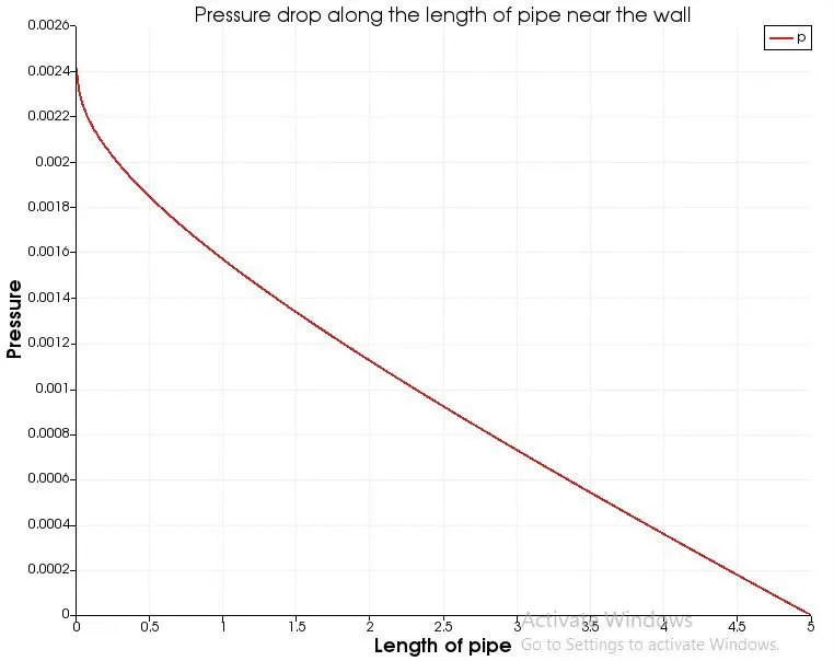
- Here the pressure is kinematic pressure = pressure/density of the fluid.
- Density of water is = 995.6 kg/m^3 at 30 degree celsius.
- From graph, kinematic pressure at x = 2.5 is 0.0009, and X= 5 is 0
- Wall shear stress value between 2.5 to 5 meters is calculated using the above relation, obtained value is 0.0044802 N/m^2.
- From the simulation graph also, it can be seen wall shear stress is 0.0035 N/m^2
- Therefore 0.0009 difference in the values of wall shear stress calculated between analytical solution and numerical solution.
Validation of fully developed flow velocity profile with its analytical profile and Validation of maximum velocity and pressure drop for fully developed flow
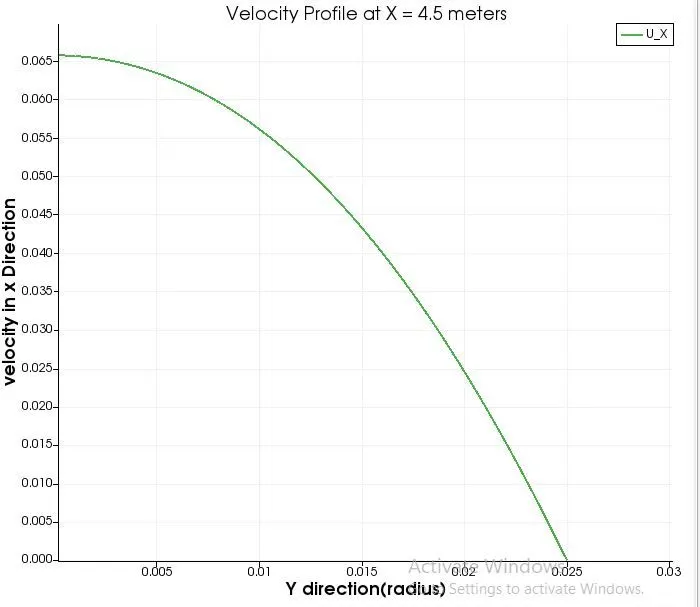
- We know that theoretically, in the fully developed region axial velocity varies parabolically in the radial direction.
- From the below graph, it can be seen, the axial velocity varying parabolically along the radial direction.
- Velocity at the inlet, calculated using Reynolds number is 0.033 m/sec. and it is the average velocity of the flow.
- Analytically we know that the maximum velocity of the flow is twice the average velocity.
- .
- Therefore maximum velocity is 0.066 m/sec.
- From the below graph, the max velocity at the center of the pipe is 0.066 m/sec, it is in good agreement with analytical maximum velocity.
- Hence it can be concluded that the numerical solution obtained is in good agreement with the analytical solution.
- From theory, as the fluid flows in a pipe due to viscous force, it increases velocity in the flow direction and at the same time pressure drops in the flow direction.
- Pressure drop at the entrance is very high and decreases gradually along with the flow and it can be seen in the below graph
- we Know that at center r = 0, u(r) =Umax
- Let's assume the flow is fully developed between 2.5meter to 5 meters.
- Here the pressure is kinematic pressure = pressure/density of the fluid.
- Density of water is = 995.6 kg/m^3 at 30 degree celsius.
- From graph, kinematic pressure at x = 2.5 is 0.0009, and X= 5 is 0
- Umax at the fully developed region is calculated using the above relation, the obtained value is 0.070 m/sec.
- From the simulation graph also, it can be seen Umax at the fully developed region is 0.066 m/sec.
- Therefore 0.004 difference in the values of Umax calculated between analytical solution and numerical solution.
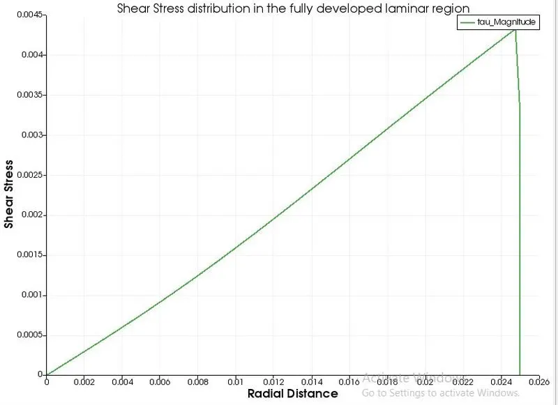
validation of wall shear stress for fully developed flow
- Theoretically, Because of the no-slip condition, velocity gradients exist in the radial direction, near the wall it is significant and velocity gradient becomes zero at the center of the flow.
- we know that shear stress near is directly proportional to velocity gradient(shear strain rate) in the radial direction(Newton law of viscosity).
- Hence shear stress near the wall is very high and decreases gradually in the radial direction and becomes zero at the center.
- It can be seen in the graph obtained from this flow simulation result.
Velocity And Pressure variation With Time
|
Velocity: |
Pressure: |
Conclusion
- The simulation is in good agreement with the analytical solution with negligible error in calculated values.
- The simulation result can be further improved, by fine meshing the flow domain,
Thank You