Week 7: Shock tube simulation project
Aim: To set up transient shock tube simulation using Converge CFD.
Aim: To perform CHT simulation on an aluminum pipe with air flowing through it.
Introduction and Theory:
A simple shock tube is a tube, rectangular or circular in cross-section, usually constructed of metal, in which gas at low pressure and gas at high pressure is separated using some form of a diaphragm. The diaphragm suddenly bursts open under predetermined conditions to produce a wave propagating through the low-pressure section. The shock that eventually forms increases the temperature and pressure of the test gas and induces a flow in the direction of the shock wave. Observations can be made in the flow behind the incident front or take advantage of the longer testing times and vastly enhanced pressures and temperatures behind the reflected wave.
The low-pressure gas, referred to as the driven gas, is subjected to the shock wave. The high-pressure gas is known as the driver gas. The corresponding sections of the tube are likewise called the driver and driven sections. The driver gas is usually chosen to have a low molecular weight, (e.g., helium or hydrogen) for safety reasons, with a high speed of sound, but maybe slightly diluted to 'tailor' interface conditions across the shock. To obtain the strongest shocks the pressure of the driven gas is well below atmospheric pressure (a partial vacuum is induced in the driven section before detonation).
The test begins with the bursting of the diaphragm. The bursting diaphragm produces a series of pressure waves, each increasing the speed of sound behind them so that they compress into a shock propagating through the driven gas. This shock wave increases the temperature and pressure of the driven gas and induces a flow in the direction of the shock wave but at a lower velocity than the lead wave. Simultaneously, a rarefaction wave, often referred to as the Prandtl-Meyer wave, travels back into the driver gas.
The interface, across which a limited degree of mixing occurs, separates driven and driver gases is referred to as the contact surface and follows, at a lower velocity, the lead wave.
Geometry Creation:
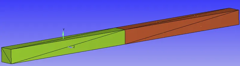
The following geometry was imported in Converge:
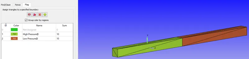
Boundary Flagging:
Case Setup:
1. Application Type: Time-based.
2. Materials
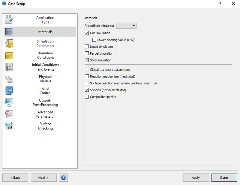
2.1. Gas simulation
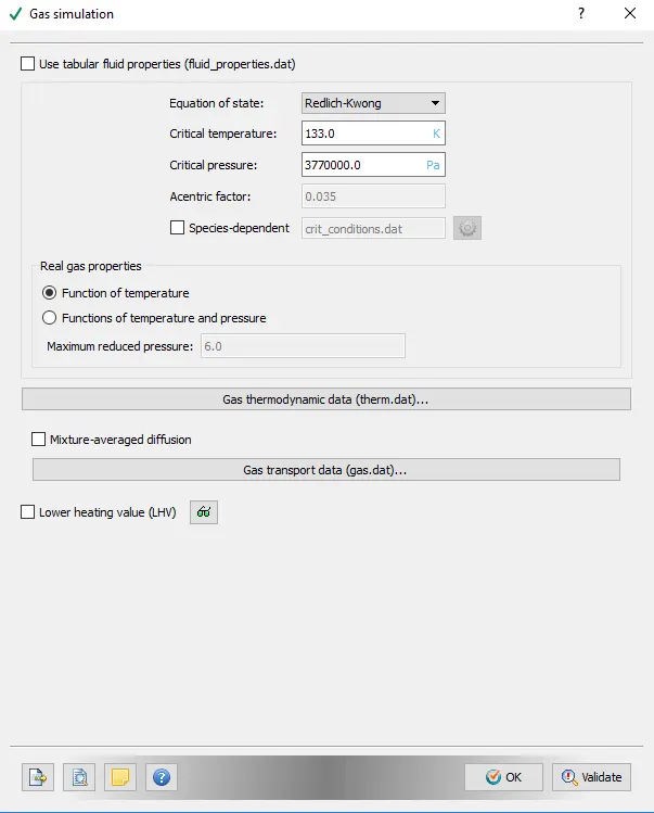
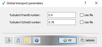
2.2. Global Transport parameters
2.3. Species
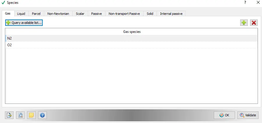
N2 and O2 are the species present in the air.
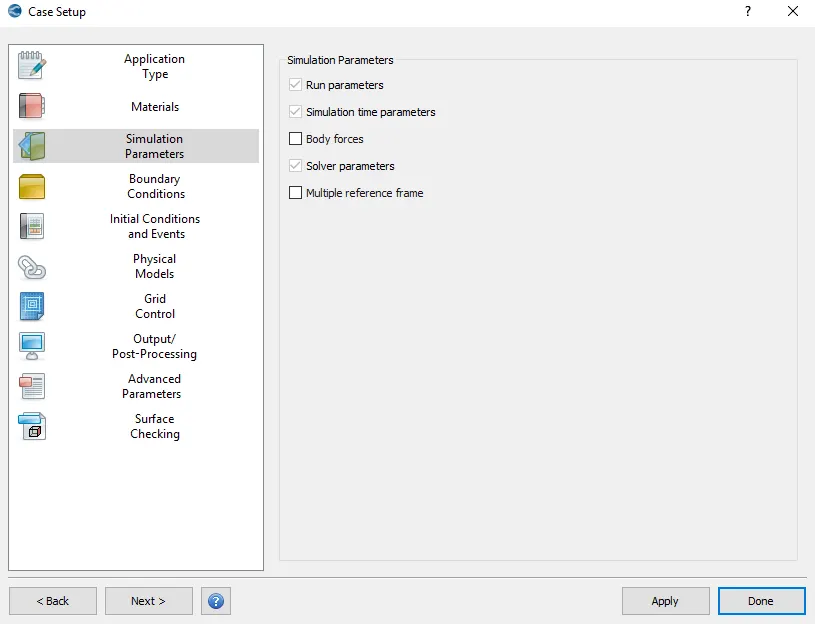
3. Simulation Parameters
3.1. Run parameters
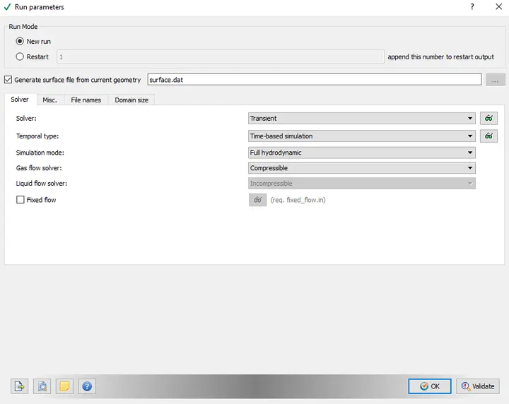
The shared memory was switched off.
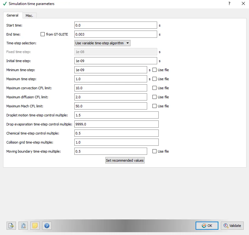
3.2. Simulation time parameters
3.3. Solver parameters
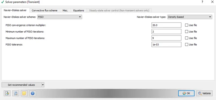
4. Boundary Conditions
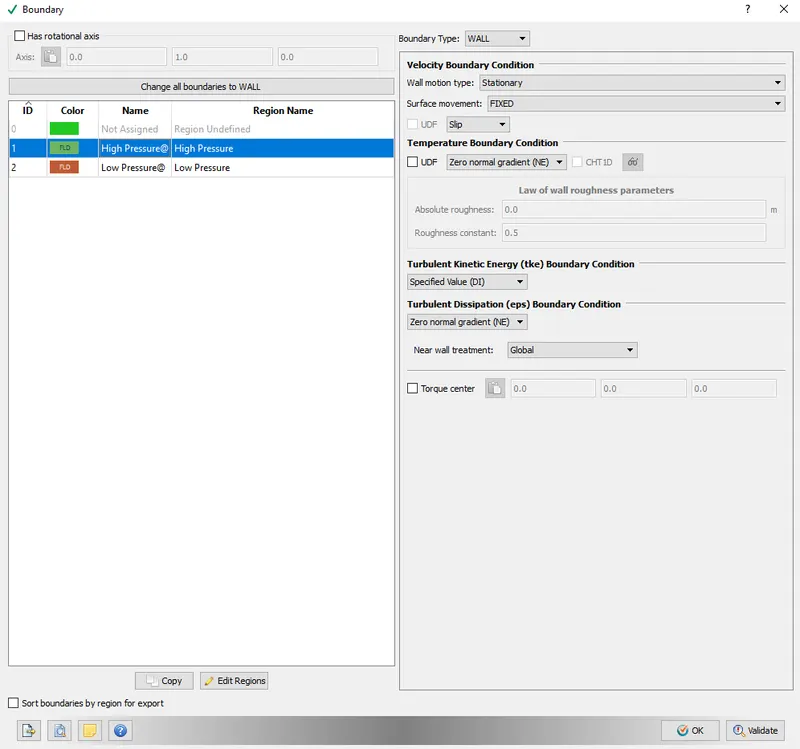
4.1. High Pressure
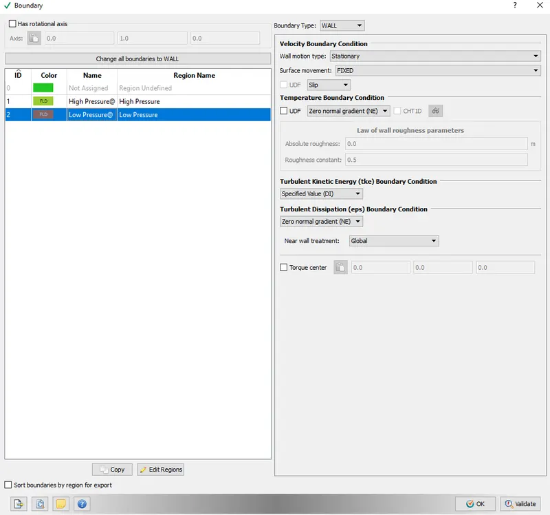
4.2. Low Pressure
5. Initial Condition and Events
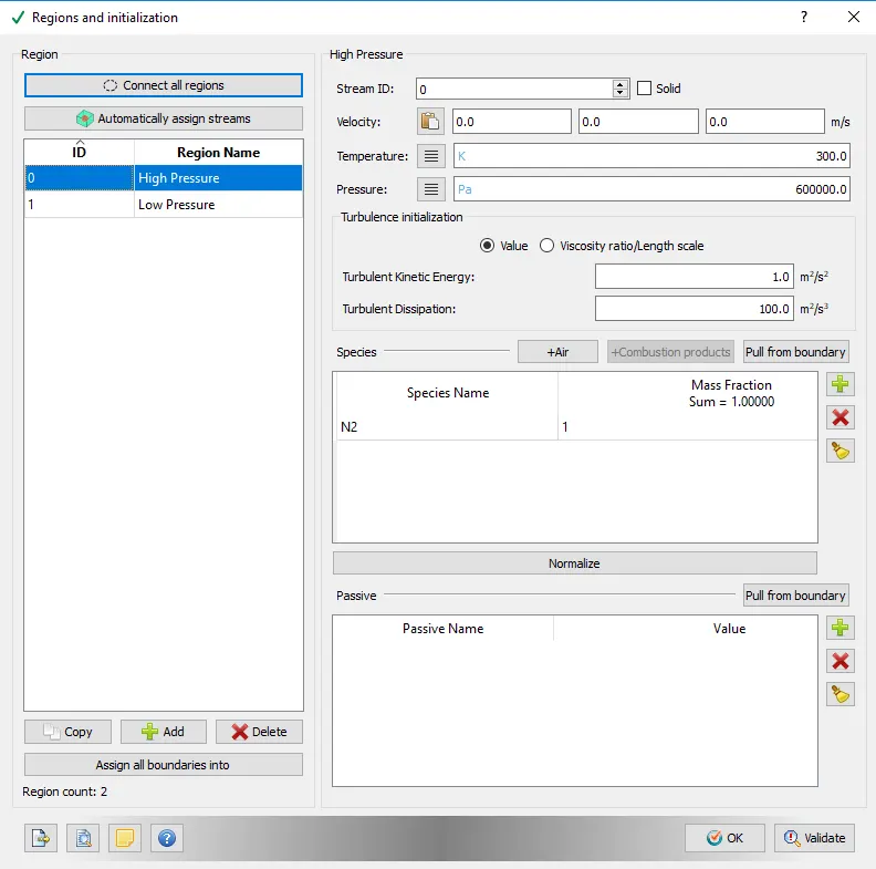
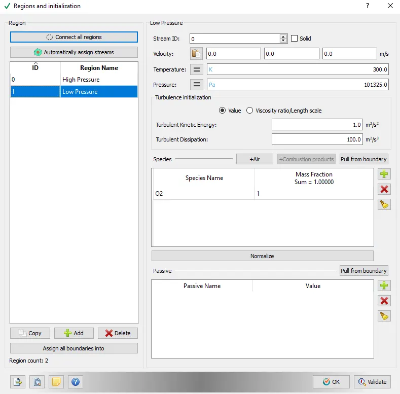
5.1. Region Initialization
Region 0 - High-Pressure region with 6 bar pressure
Region 0 - Low-Pressure region with atmospheric pressure.
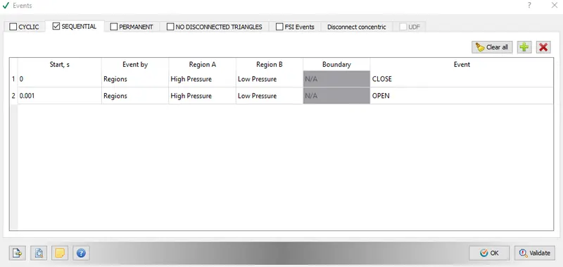
5.2 Events
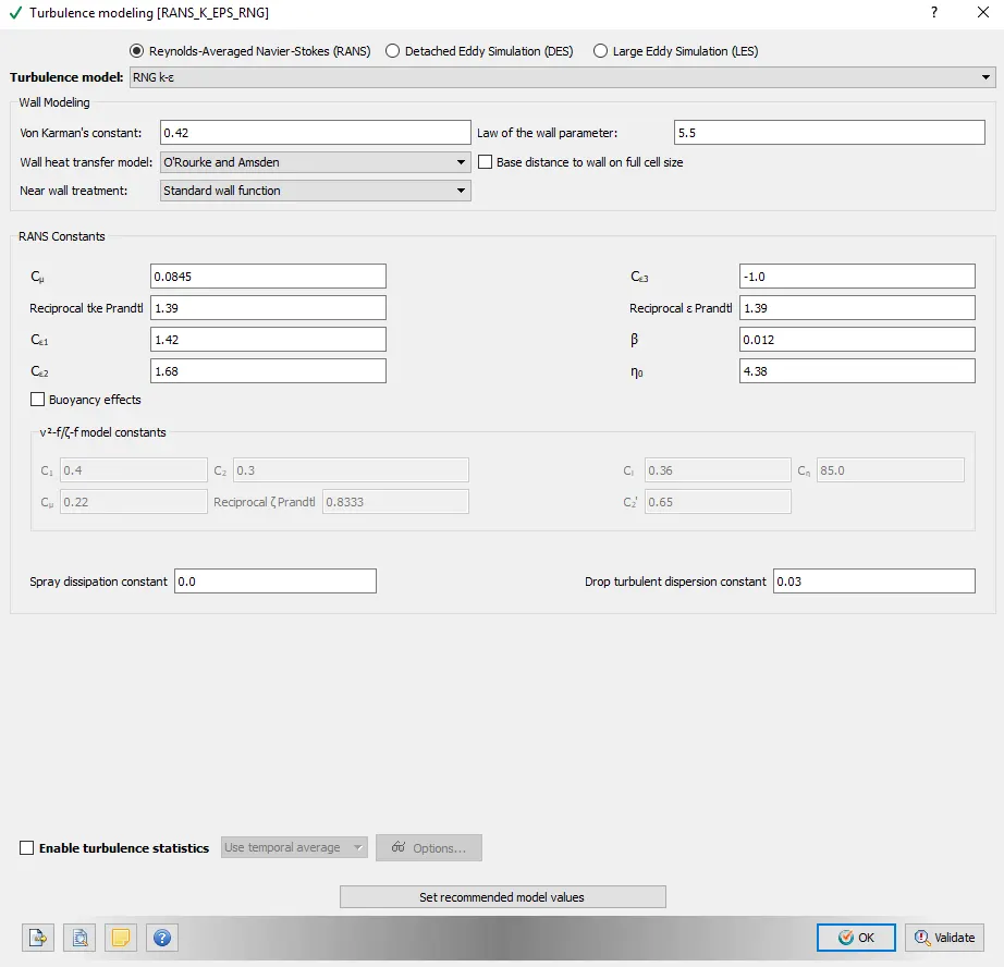
6. Turbulence modeling:
8. Grid Control
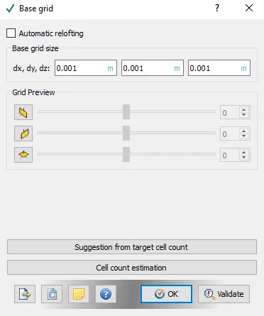
8.1. Base Grid
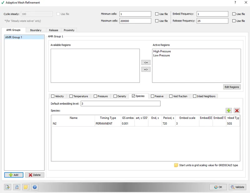
8.2. Adaptive Mesh Refinement
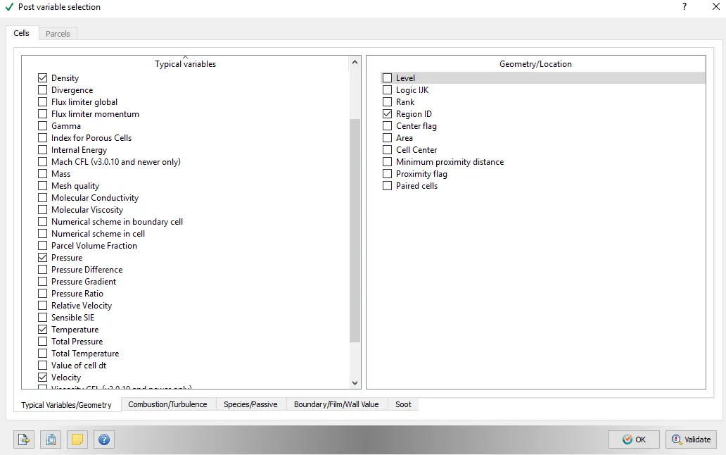
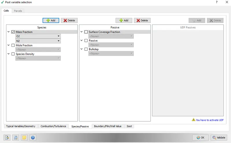
9. Output variables
9. Output files
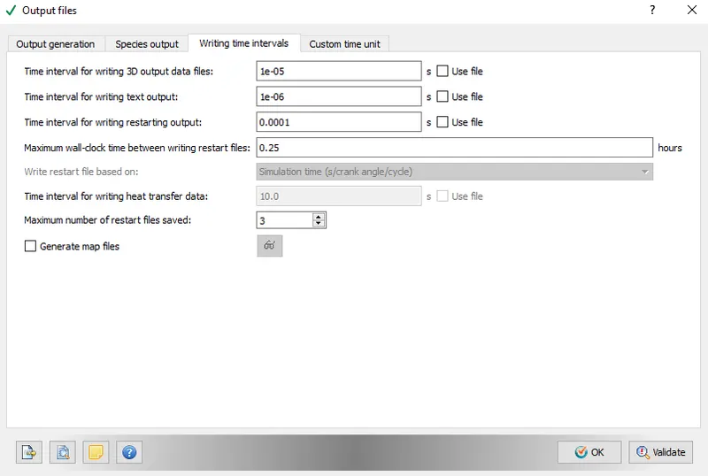
The input files were exported to a file and using the Cygwin command line, we used converge-intelmpi solver to run a parallel simulation with 4 processors.
Using the post-processing tools, the output files obtained were converted into Ensight file type which can be then opened by ParaView.
Results:
Element size = 1mm
Mesh:
The parameter for AMR is species mass fraction, so when a change greater than 0.001 is detected, there is mesh refinement.
Pressure plot:
1. Pressure plot in separate regions
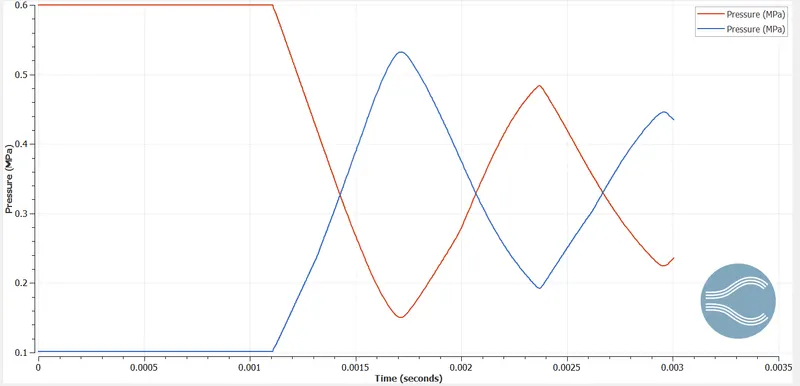
Red Line denotes Pressure in region 0 (high-pressure region).
Blue Line denotes pressure in region 1 (low-pressure region).
The pressure in region 0 decreases initially and then increases in a cyclic manner, because of the back and forth shock propagation. However, the amplitude decreases after every wavelength.
Similarly, The pressure in region 1 increases initially and then decreases in a cyclic manner, because of the back and forth shock propagation. However, the amplitude decreases after every wavelength.
After a certain period of time, the shock will be dissipated and the system will be in equilibrium.
2. Pressure plot in the entire domain
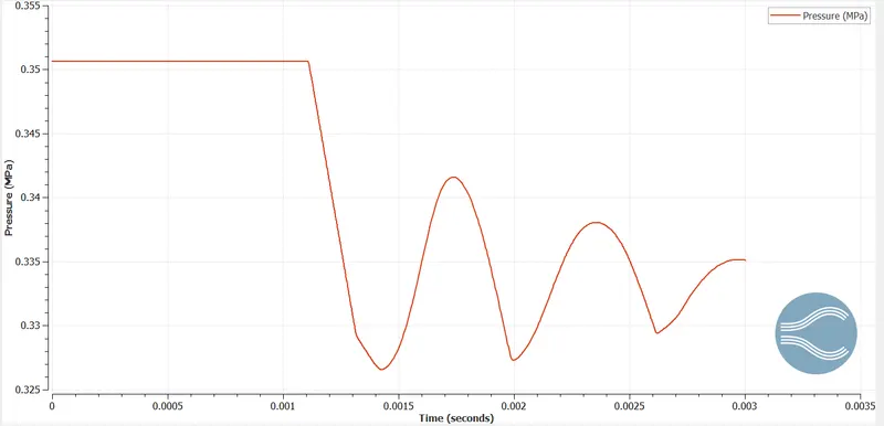
The pressure in the entire domain decreases and increases in a cyclic manner. The pressure will keep on decreasing until equilibrium is attained.
Temperature plot:
1. Temperature plot in separate regions
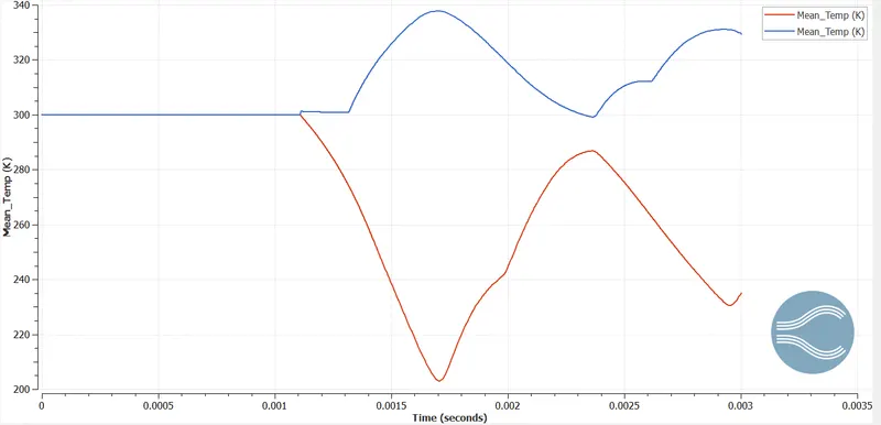
Red Line denotes Temperature in region 0 (high-pressure region).
Blue Line denotes Temperature in region 1 (low-pressure region).
The temperature in region 0 decreases initially and then increases in a cyclic manner, because of the back and forth shock propagation. However, the amplitude decreases after every wavelength.
Similarly, The temperature in region 1 increases initially and then decreases in a cyclic manner, because of the back and forth shock propagation. However, the amplitude decreases after every wavelength.
After a certain period of time, the shock will be dissipated and the system will be in equilibrium.
2. Temperature plot in the entire domain
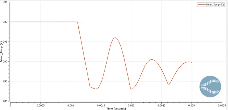
The temperature in the entire domain decreases and increases in a cyclic manner. The temperature will keep on decreasing until equilibrium is attained.
Mass fraction plot:
1. Mass fraction of N2 in the region 0
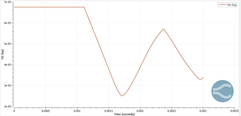
The mass fraction of N2 decreases in region 0 initially since it gets expanded into the low-pressure domain, however when the shock propagates back, the N2 species is pushed back to the high-pressure domain, hence we observe the cyclic behavior.
2. Mass fraction of O2 in the region 1
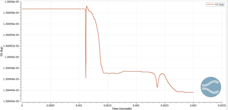
The mass fraction of O2 decreases in the low-pressure domain since the high-pressure gas expands into the low-pressure domain. However, change isn't of much magnitude.
Cells as a function of time:
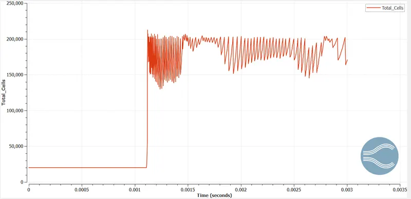
The cell count keeps on changing, which depends on the AMR criteria of species mass fraction in the domain. After the diaphragm is opened at the interface, we can observe the cell count shoots up, as N2 and O2 start mixing and then depending on the movement of the species, further mesh refinement was captured.
Animation:
1. Pressure Animation
The pressure animation clearly depicts how the pressure increases and decreases in a cyclic manner in both the regions due to the back and forth motion of the shock waves.
2. Temperature Animation
The temperature animation clearly depicts how the temperature increases in the direction of the shock wave i.e. towards region 1. It tries to shift towards region 0 during the backpropagation of shock wave, however it majorly stays in region 1.
The mass fraction animation clearly depicts how the mass fraction increases towards region 1 as the high-pressure gas expands into the low-pressure region. The back and forth movement of shock waves try to push the N2 species back and forth the region.
Conclusion:
A Transient shock tube simulation was conducted on Converge CFD and its effect on the pressure and temperature of the domain was studied. Also, the variation of cell count due to the AMR was observed.