Week 6: Conjugate Heat Transfer Simulation
Aim: To perform CHT simulation on an aluminum pipe with air flowing through it.
Introduction and Theory: CHT(Conjugate Heat Transfer) corresponds to the heat transfer in solids and heat transfer in fluids. In solids, conduction often dominates and in fluids, convection dominates.CHT analysis allows us to analyze heat transfer between a solid domain and a fluid domain. We can simulate the flow of fluids of any velocity, temperature, physical and chemical property through or around a solid of any shape, size, physical, and chemical property. This, allows us to analyze the heat transfer characteristics at the interface between both the domains.
CHT analysis is beneficial in accurately predicting solid temperatures and heat transfer capabilities in engineering devices. Using CHT analysis, engineers can optimize the thermal characteristics of the product.
Applications: HVAC, Internal Combustion Engine, Gas Turbines, Heat Exchangers
Calculation of Inlet Velocity:
Given Reynolds Number = 7000
The density of air (@300K and 1 atm) = 1.1766 `(kg)/m^3`
Dynamic Viscosity (@300K and 1 atm) = 0.00001846 `(kg)/(ms)`
Kinematic Viscosity = `v` = `mu/rho` = 1.56893e-05 `m^2/s`
Pipe Inner diameter = D = 0.03 m
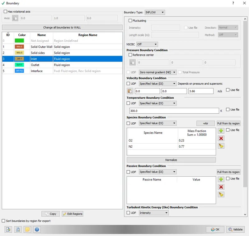
Average flow velocity = `(Re*mu)/(rho*D)` = 3.66 m/s
Skin friction drag coefficient = `C_f` = 0.0576`*(Re)^(-1/5) `= 0.00980399
Wall shear stress, `tau_w = C_f*(rho*v^2)/2` = 0.077296708 `N/m^2`
Frictional Velocity = `u_t` = `root()(tau_w/rho)` = 0.256310311 m/s
For Y+ = 30,
First cell center height = `Y_+* v/u_t` = 0.001836363891 m
First cell height = 0.0036727 m
Hence we can start with 4mm as the first cell height, and then proceed with grid independence study with finer refined meshes.
Geometry Creation:
The following geometry was created in Converge:
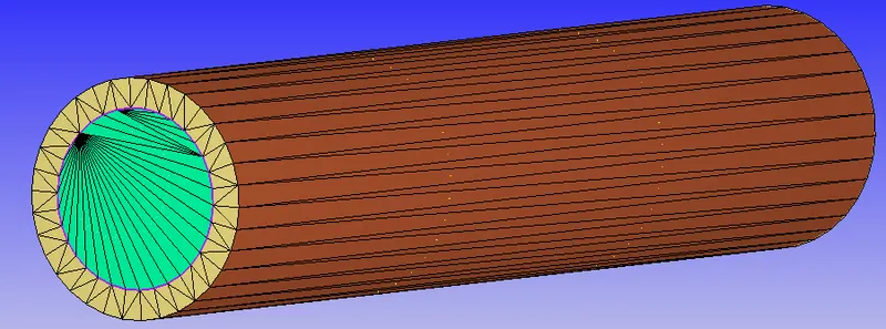
The geometry was repaired to remove the issue of Intersecting edges. The non-manifold issue is there, however, it cannot be removed for CHT simulations and can be ignored. Make sure all the normals are pointing towards the fluid domain. Also, the inlet and outlet surfaces were patched using the patch tool.
Boundary Flagging:
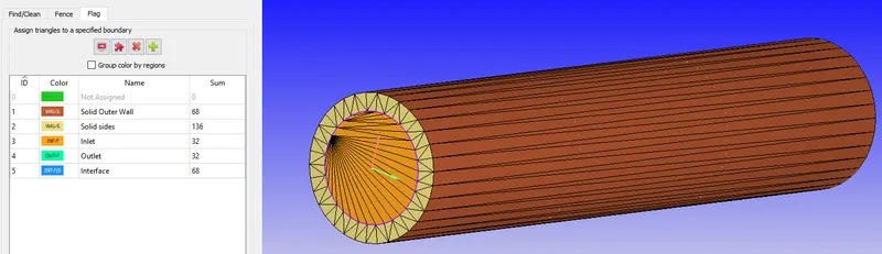
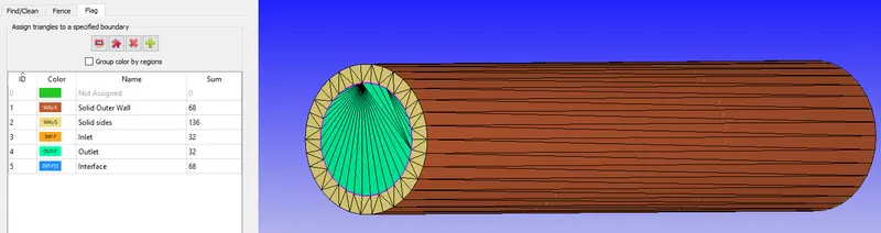
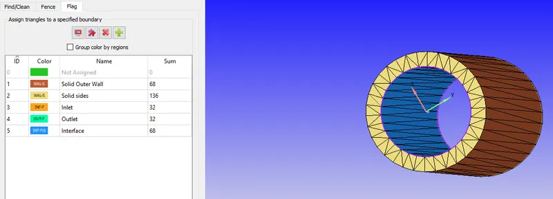
Case Setup:
1. Application Type: Time-based.
2. Materials
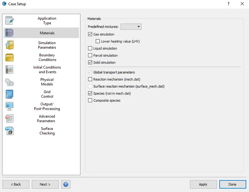
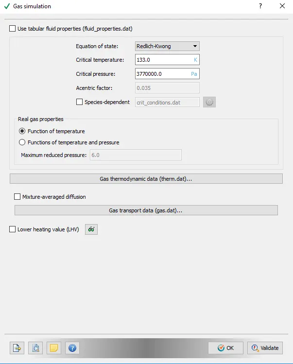
2.1. Gas simulation
2.2. Solid simulation
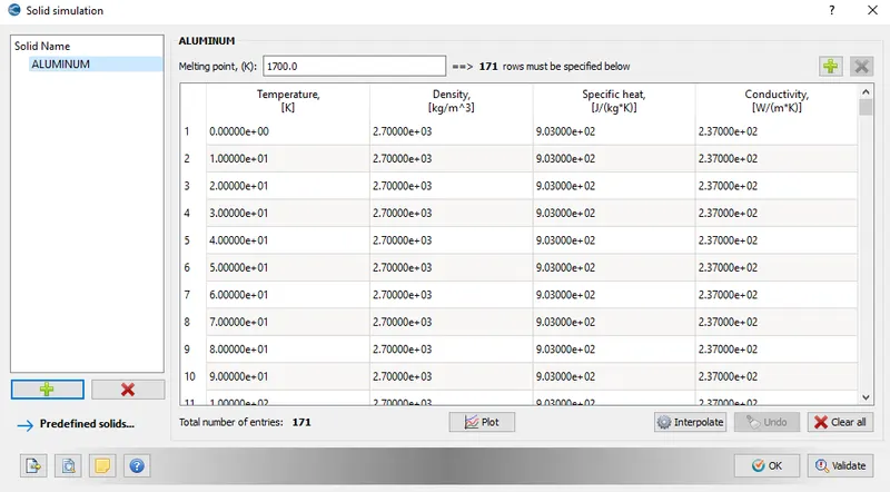
Predefined material aluminum is chosen for the solid pipe.
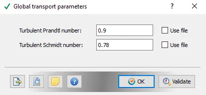
2.3. Global Transport parameters
2.4. Species
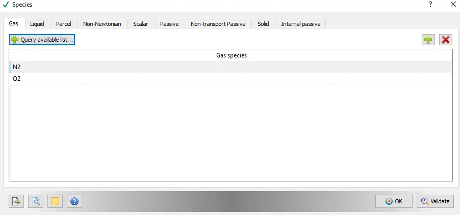
N2 and O2 are the species present in the air.
3. Simulation Parameters
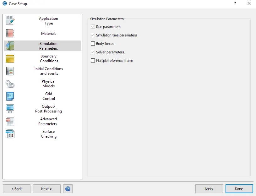
3.1. Run parameters
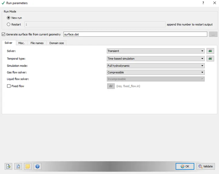
The shared memory was switched off.
3.2. Simulation time parameters
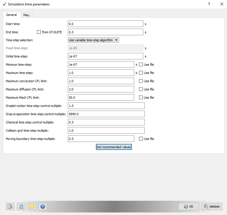
3.3. Solver parameters
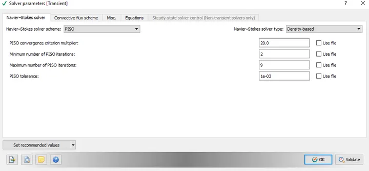
4. Boundary Conditions
4.1. Solid Outer Wall
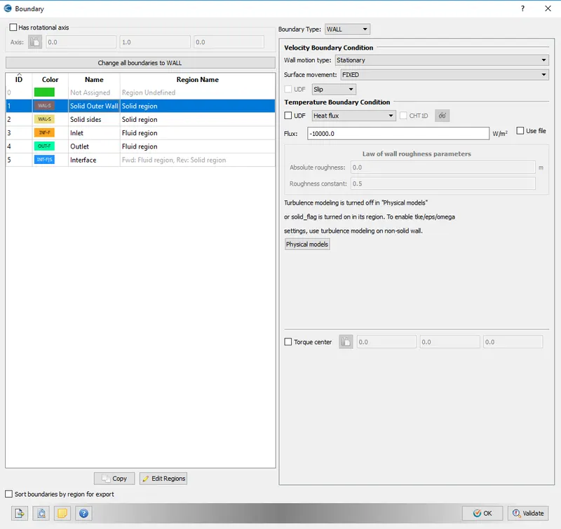
The -ve sign of heat flux indicates that the flux is directed inside the domain.
4.2. Solid sides
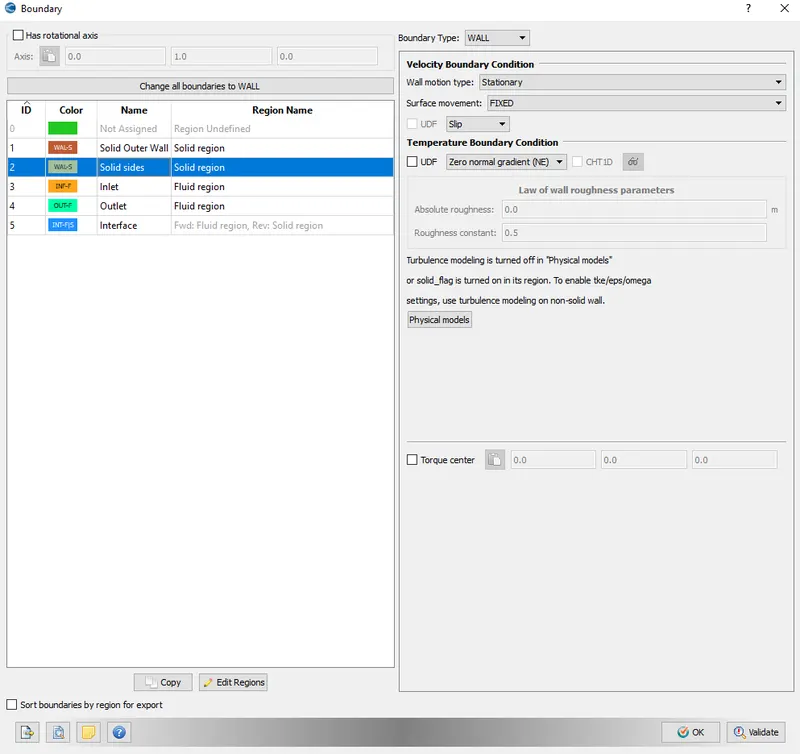
4.3. Inlet
4.4. Outlet
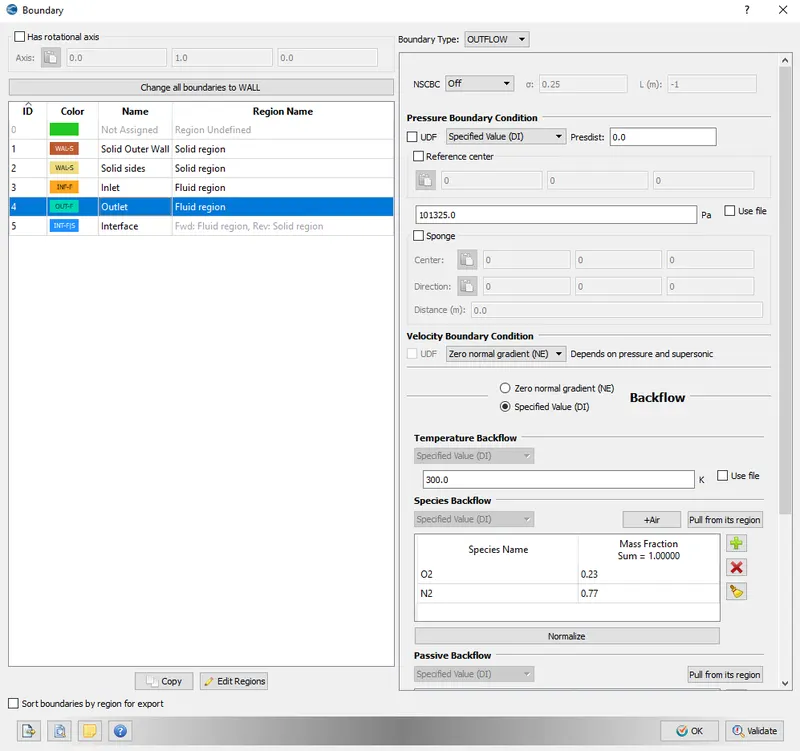
4.5. Interface
4.5.1. Forward side
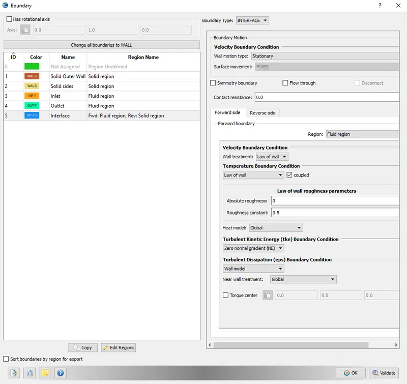
The forward side denotes the region towards which the normal point at which is the fluid region.
4.5.2. Reverse side
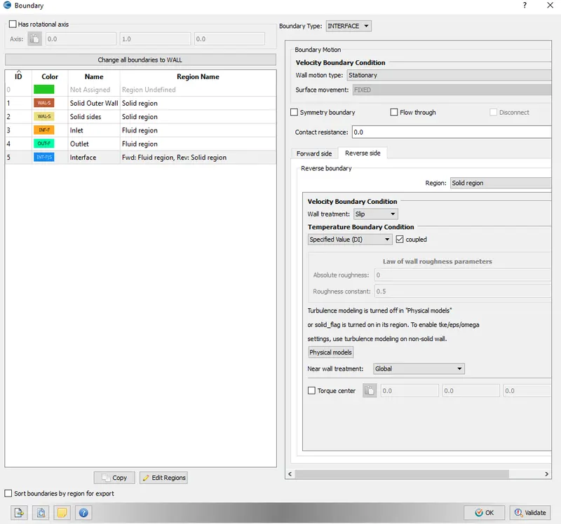
The reverse side denotes the region opposite of which the normal point at which is the solid region.
5. Region Initialization
5.1. Fluid region
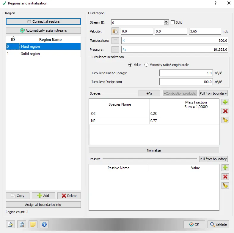
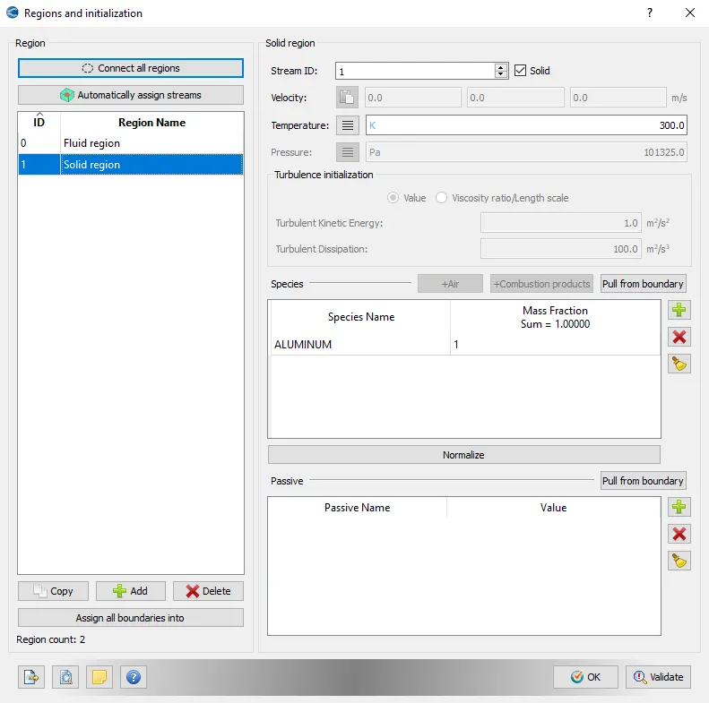
5.2. Solid region
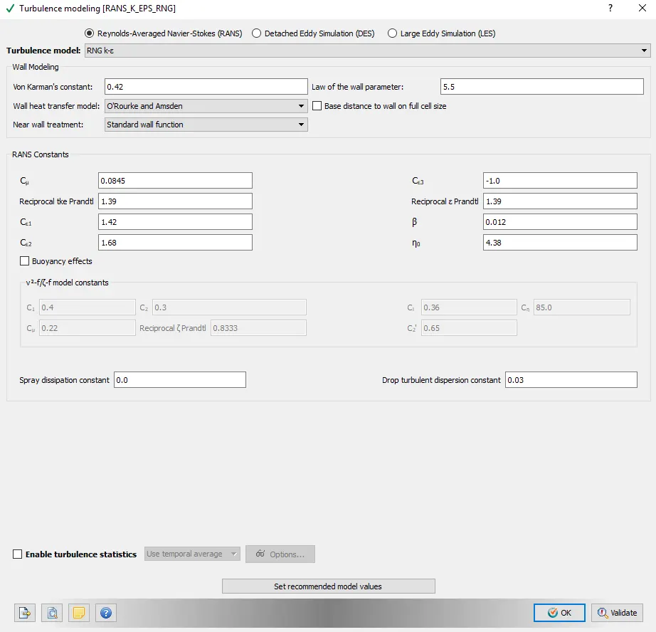
6. Turbulence modeling:
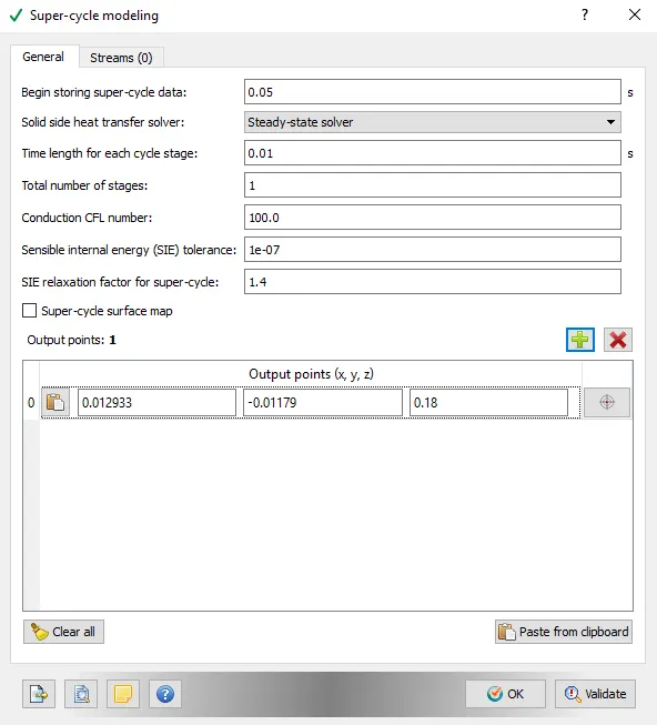
7. Super-cycle modeling
8. Grid Control
8.1. Base Grid
Case 1: dx, dy, dz= 0.004 m
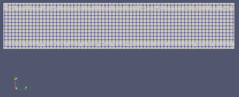
Case 2: dx, dy, dz= 0.003 m
Case 3: dx, dy, dz= 0.002 m
9. Output variables
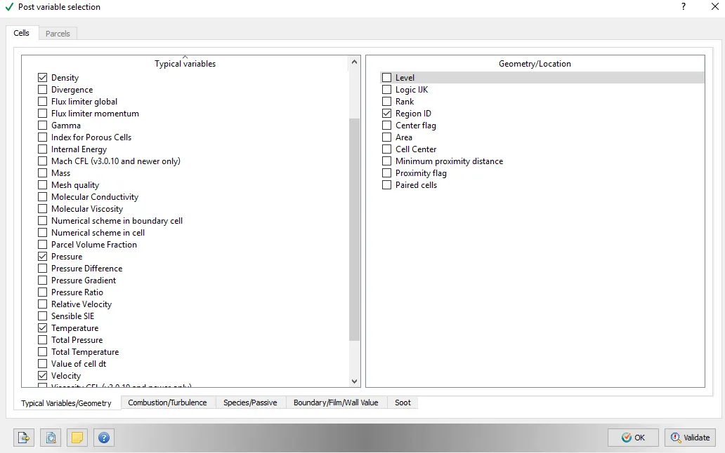
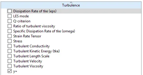
Add y+ to the output variables.
9. Output files
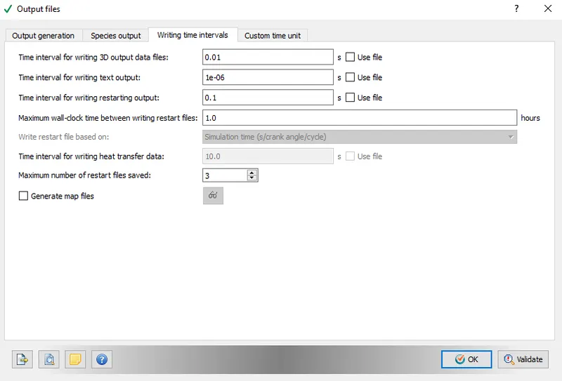
The input files were exported to a file and using the Cygwin command line, we used converge-intelmpi solver to run a parallel simulation with 4 processors.
Using the post-processing tools, the output files obtained were converted into Ensight file type which can be then opened by ParaView.
Grid Independence Test:
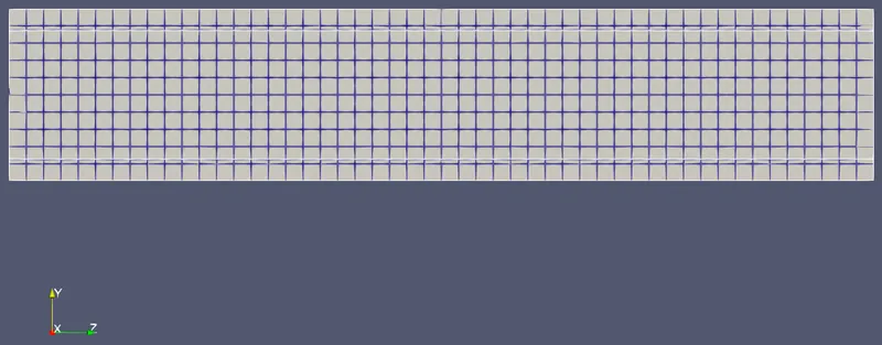
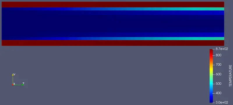
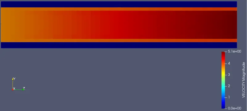
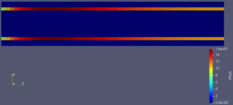
Case 1: Element size = 4mm
Mesh:
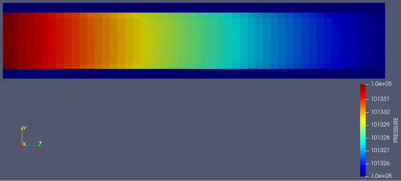
Pressure contour:
Temperature contour:
Velocity contour:
Y+ contour:
The mean temperature at Outlet plot:
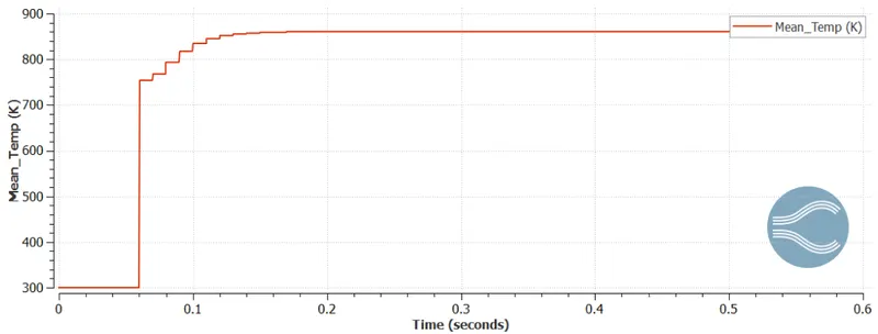
The mean temperature at the outlet is 860.59
Case 2: Element size = 3mm
Mesh:
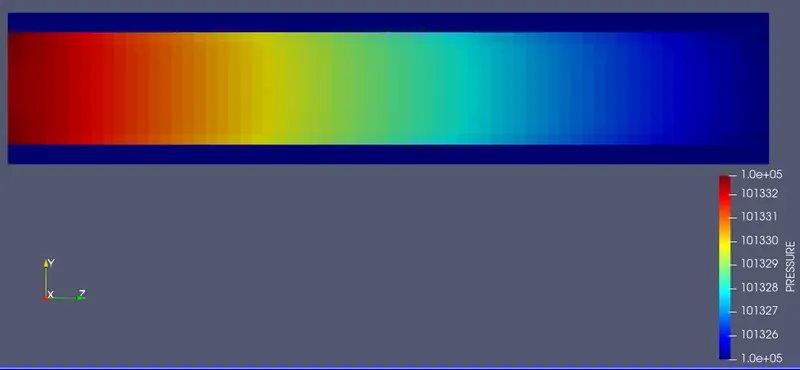
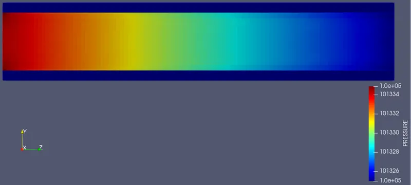
Pressure contour:
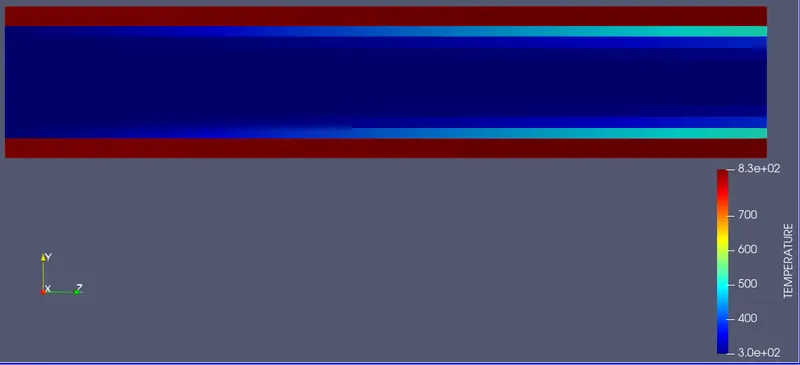
Temperature contour:
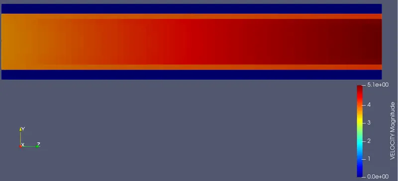
Velocity contour:
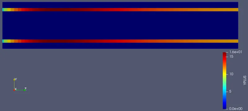
Y+ contour:
The mean temperature at Outlet plot:
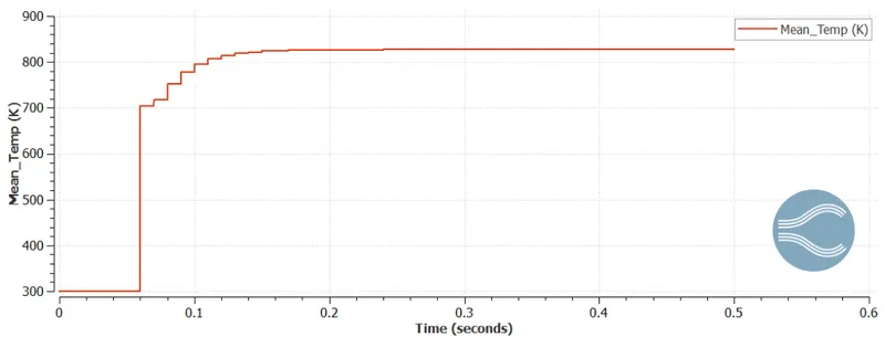
The mean temperature at the outlet is 827.08
Case 3: Element size = 2mm
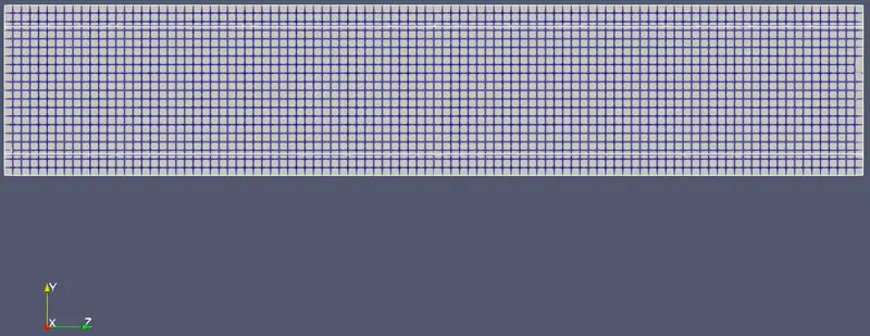
Mesh:
Pressure contour:
Temperature contour:
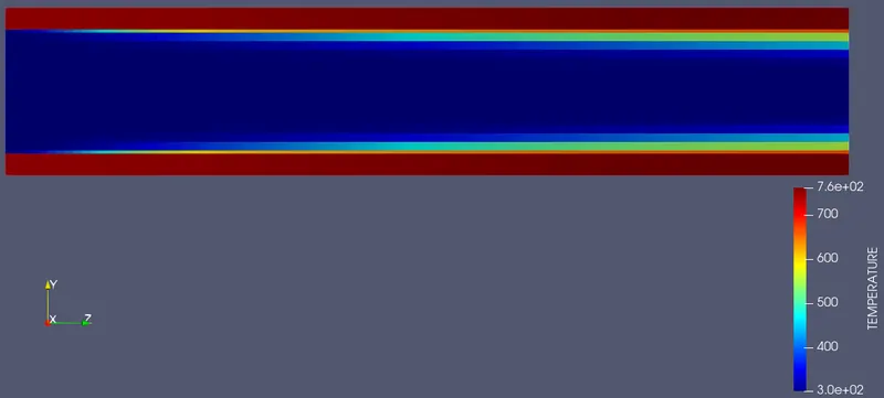
Velocity contour:
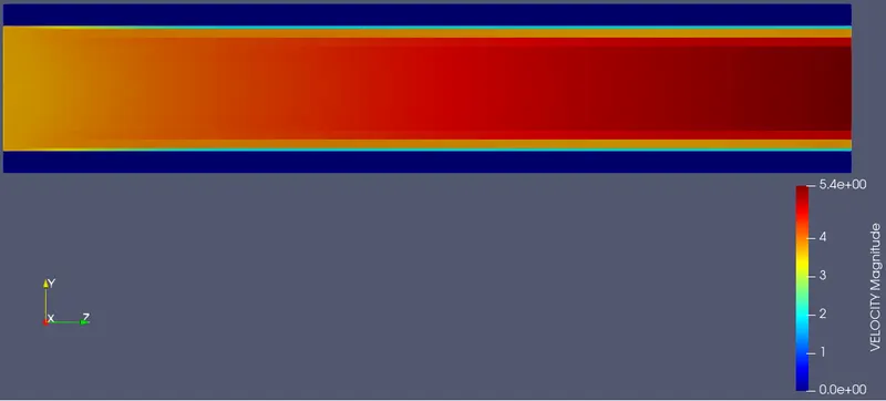
Y+ contour:
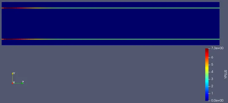
The mean temperature at Outlet plot:
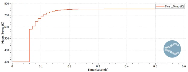
The mean temperature at the outlet is 753.6 K.
Effect of supercycle stage interval:
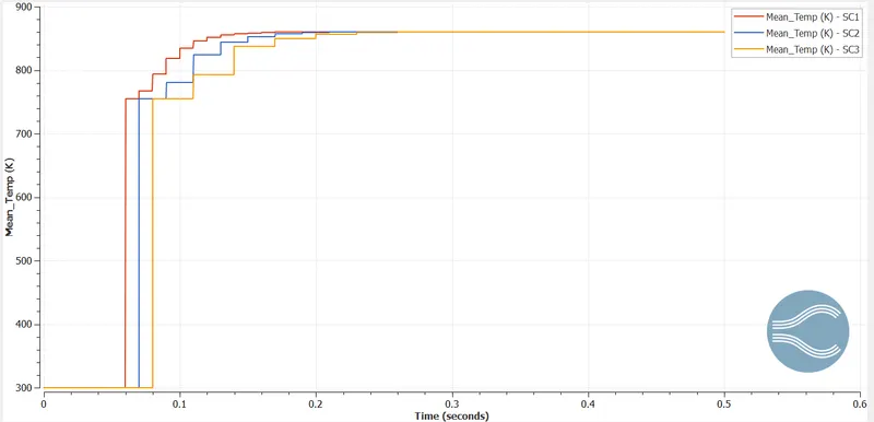
SC1 - SuperCycle stage interval is 0.01
SC2 - SuperCycle stage interval is 0.02
SC3 - SuperCycle stage interval is 0.03
All the above intervals are applied for the base mesh.
The average temperature value at the outlet is 826.5 K.
During super-cycling, after every stage interval, the main solver is paused and only the solid solver is continued until the steady-state is reached. This helps us to speed up the process because generally fluids and solids have different heat transfer rates and hence solving them at the same time-step will take more time to obtain convergence. So, the lower the stage interval, the more frequently the solid solver is solved and hence we obtain faster convergence. The above graph of the mean temperature at the outlet depicts the explanation.
The simulation time for SC1 is 268.92 s
The simulation time for SC2 is 284.12 s
The simulation time for SC3 is 296.66 s
Hence, we can observe that reducing the Stage-interval reduces the simulation time and also helps us to achieve quicker convergence.
Animation:
1. Pressure Animation
2. Temperature Animation
3. Velocity Animation
Conclusion:
1. Y+ values decrease with decreasing mesh size as expected.
2. The value of the mean temperature at the outlet decreases with decreasing mesh size.
3. The mean temperature value of 753.6 K for 2mm can be considered to be more accurate to actual results than the mesh sizes of 4 and 3 mm.
4. The pressure across the pipe reduces as expected.