Week 10: Project 1 - FULL HYDRO case set up (PFI)

Aim: Simulation of a Full-Hydrodynamic Port-Fuel Injection engine in Converge CFD.

Introduction and Theory:

Fuel injection is the introduction of fuel in an IC engine, most commonly automotive engines, through an injector. Fuel injection was replaced by carburetors from the 1990s onward. The main difference between carburetion and fuel injection is that fuel injection atomizes the fuel through a small nozzle under high pressure, while a carburetor relies on suction created by intake air accelerated through a Venturi tube to draw the fuel into the airstream. There are several benefits of using the fuel injection system. Like digital electronic fuel injection systems optimize power output, efficiency, emission performance competing objectives more effectively and consistently than earlier fuel delivery systems.

Case Setup:

Step 1: Importing Geometry

The following geometry was imported into Converge.

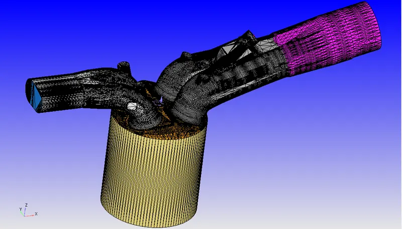
Boundary flagged components:

1. Piston

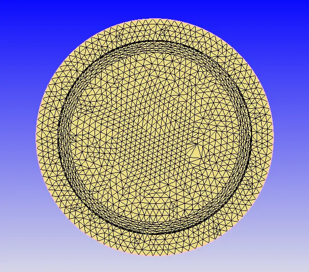
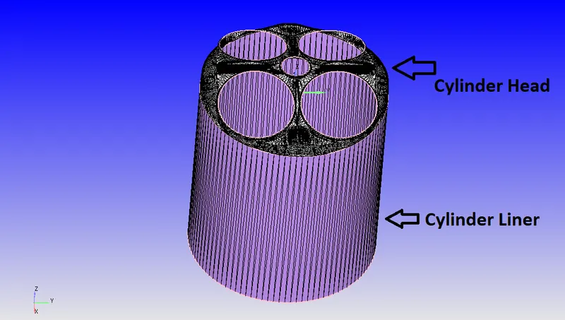
2. Cylinder Head and Cylinder Liner

3. Intake Valve 

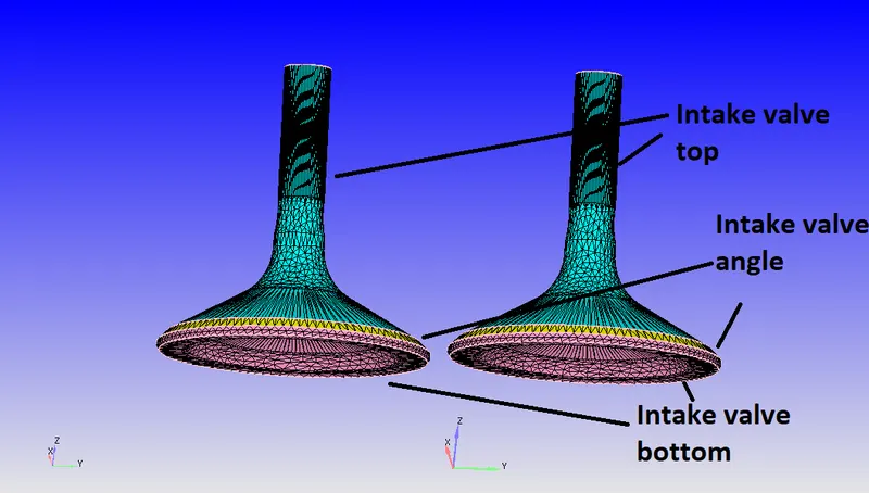
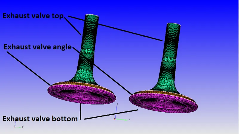
4. Exhaust valve

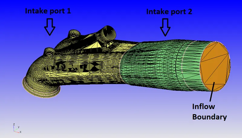
5. Intake port and inflow boundary

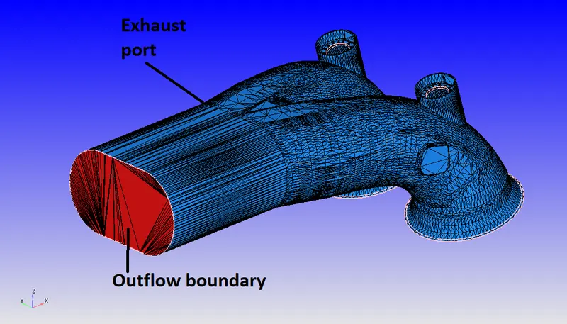
6. Exhaust port and outflow boundary

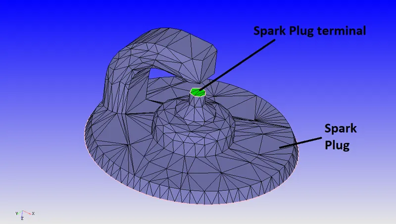
7. Spark plug and Spark plug terminal

Case Setup:

1. Application Type: Crank angle-based IC engine.

2. Materials

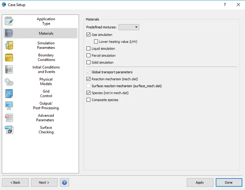
2.1. Gas simulation

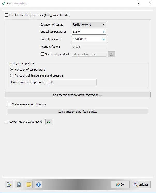
Gas thermodynamic data was imported using the file provided.

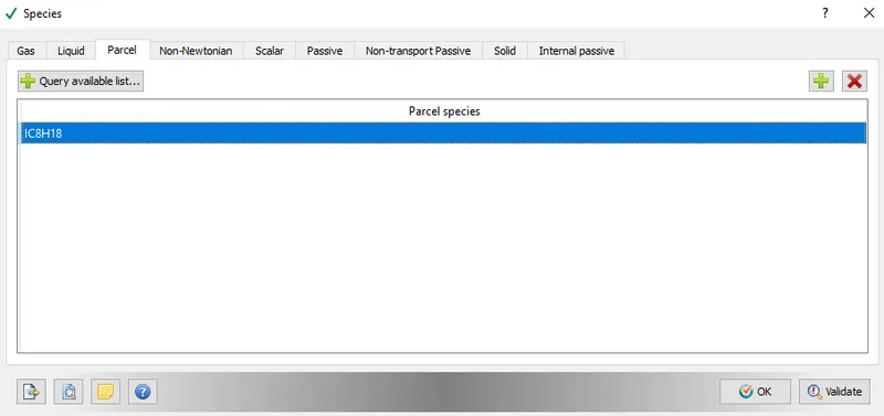
2.2 Parcel simulation

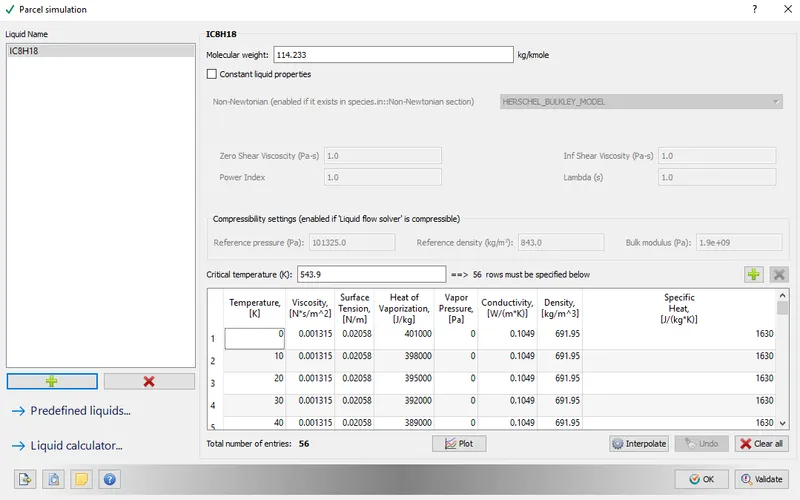
Parcel simulation is required to model fuel drops as Lagrangian parcels. When fuel is injected in its liquid form at high velocity and pressure, there is a drag force that breaks down the liquid fuel into parcels(say primary parcels), which are further broken down into subsequent smaller parcels. As the parcels move with high velocity its size decreases due to fuel evaporation. Hence we have initialized iso-octane as the parcel species here. (It has properties similar to gasoline)

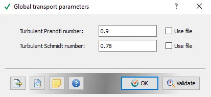
2.3. Global Transport parameters

2.4.Reaction mechanism

Species taking part in the reaction are shown below.

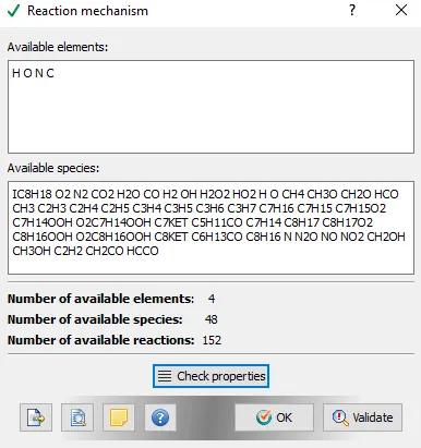
Mech.dat data was imported.

2.5. Species

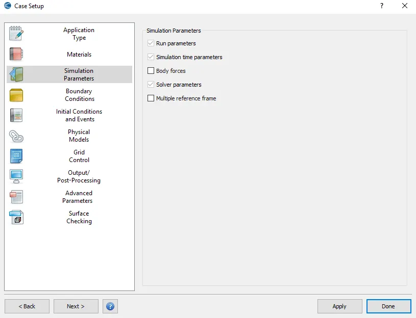
3. Simulation Parameters

3.1. Run parameters

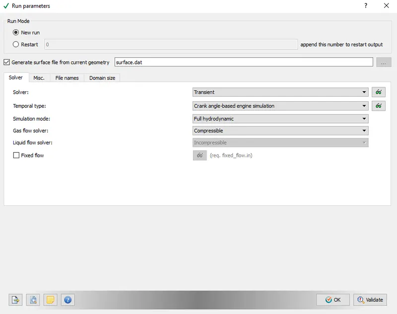
Shared memory was switched off.

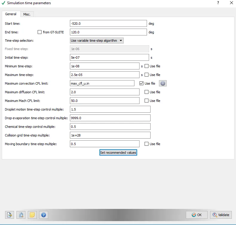
3.2. Simulation time parameters

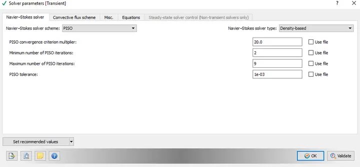
3.3. Solver parameters

4. Boundary Conditions

4.1. Piston

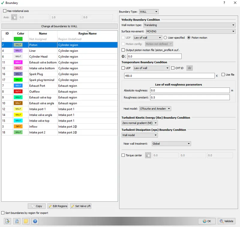
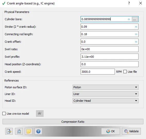
Converge uses slider-crank mechanism properties provided to calculate piston motion velocity.

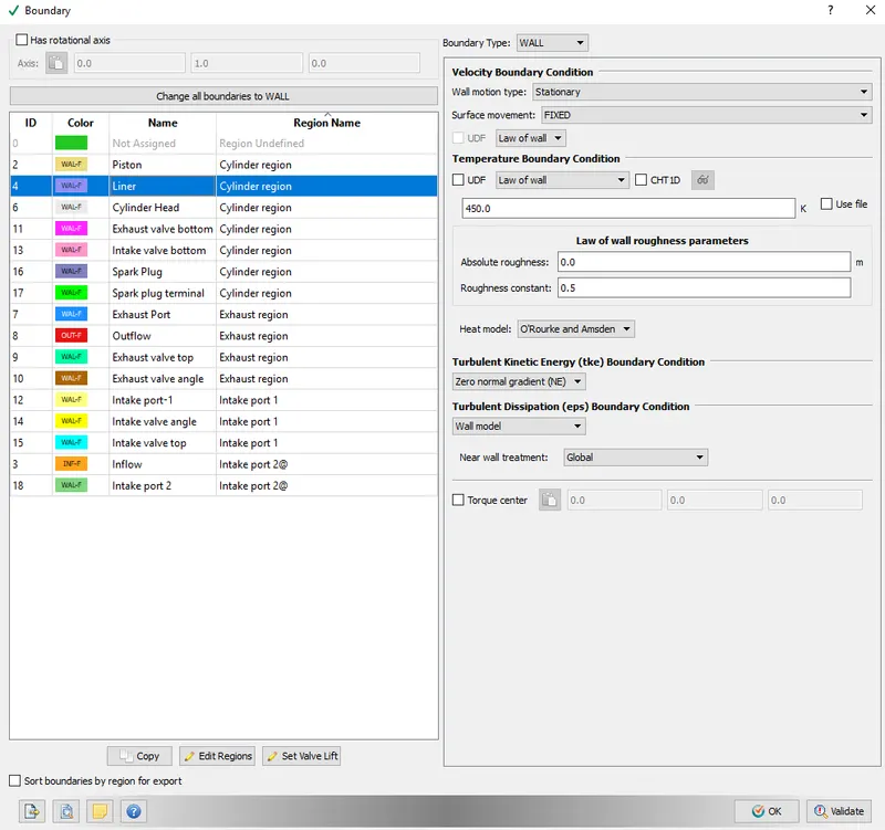
4.2. Liner

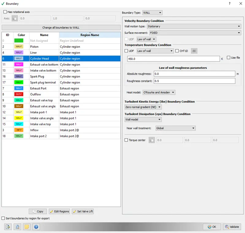
4.3. Cylinder Head

4.4. Exhaust valve bottom

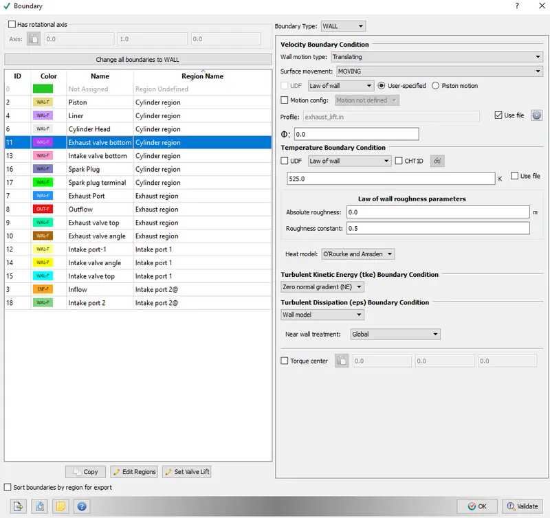
The exhaust valve motion file was imported.

4.5. Intake valve bottom

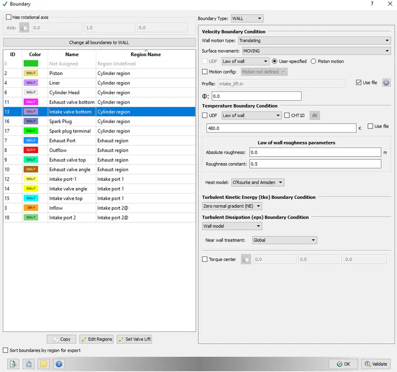
The intake valve motion file was imported.

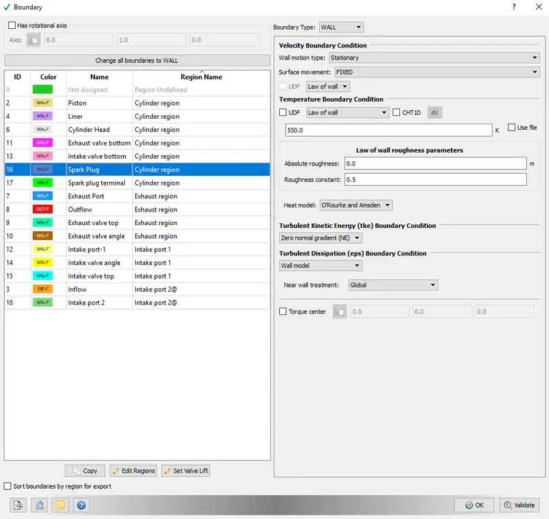
4.6. Spark Plug

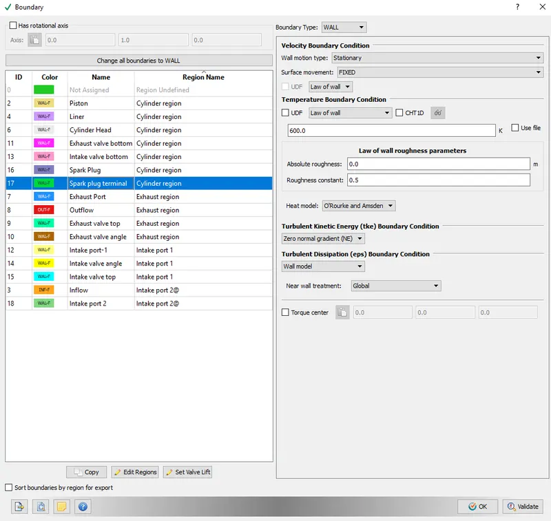
4.7. Spark plug terminal

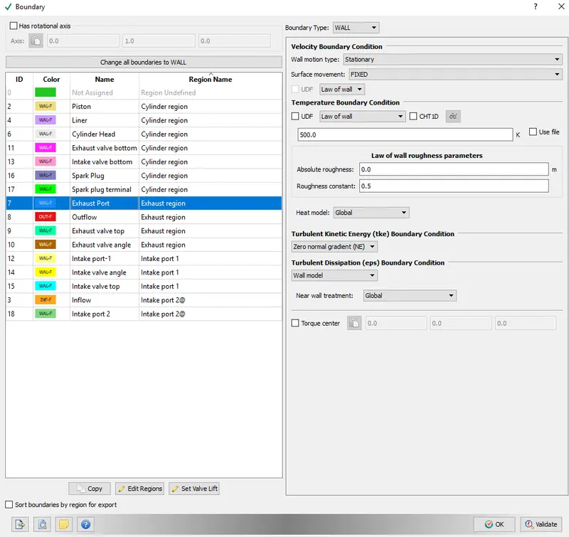
4.8. Exhaust port

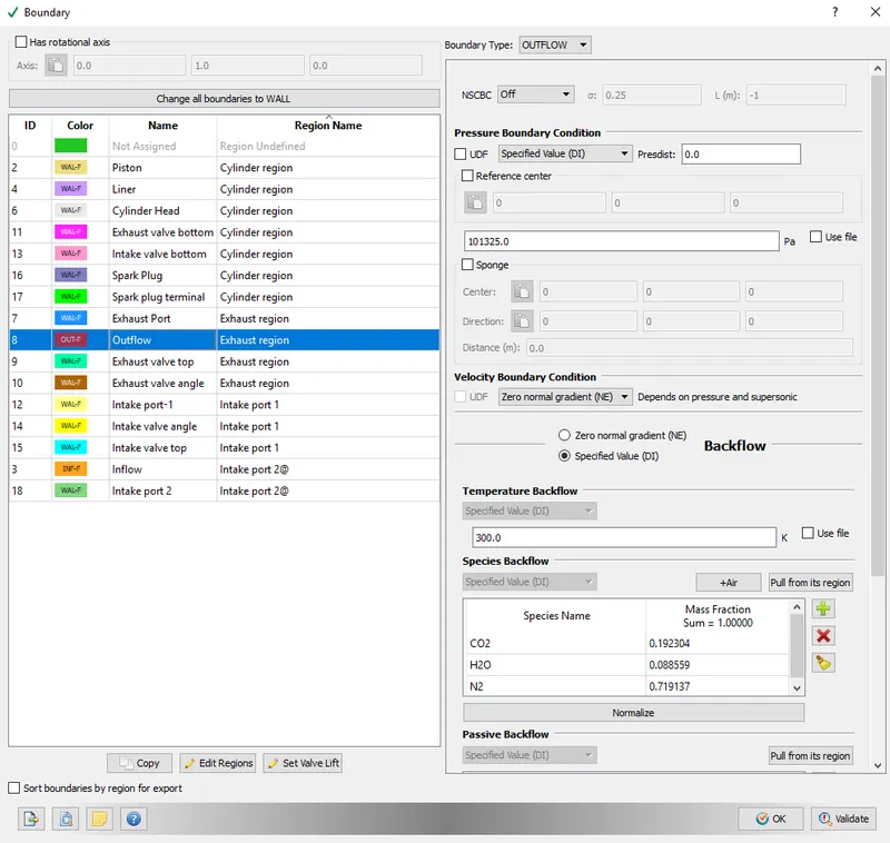
4.9. Outflow

4.10. Exhaust valve top

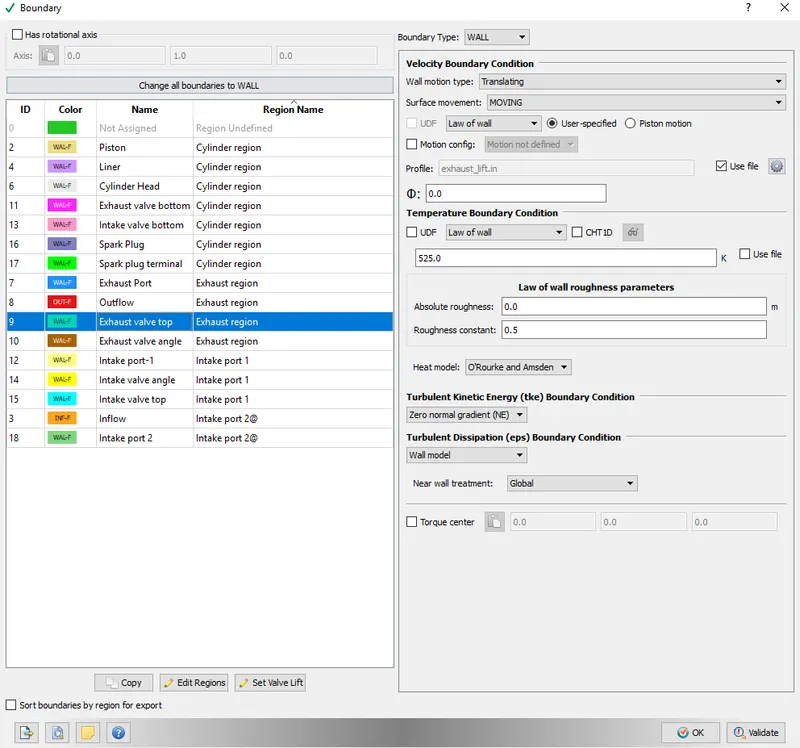
The exhaust valve motion file was imported.

4.11. Exhaust valve angle

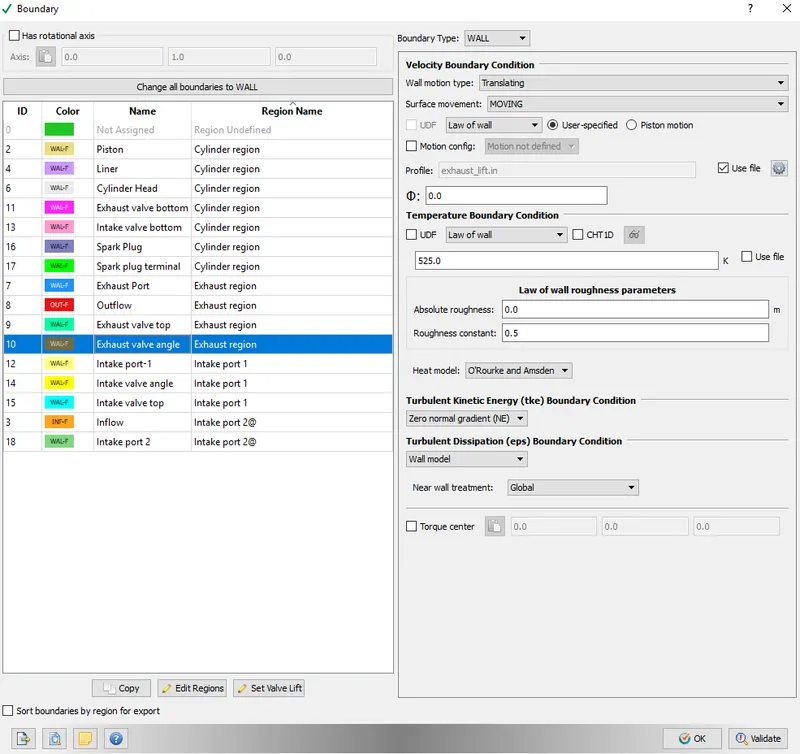
The exhaust valve motion file was imported.

4.12. Intake port-1

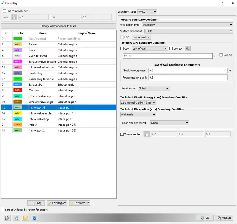
4.13. Intake valve angle

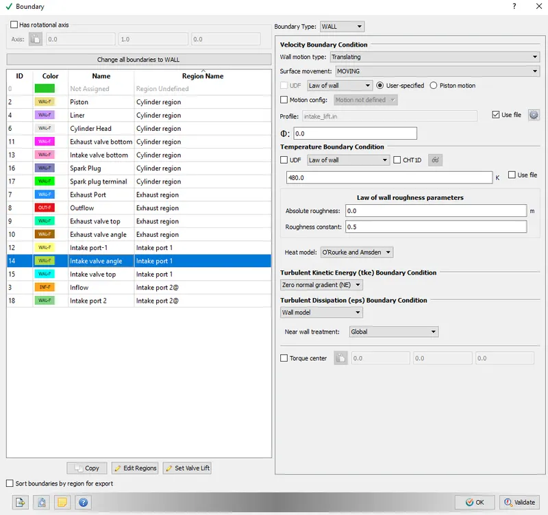
The intake valve motion file was imported.

4.14. Intake valve top

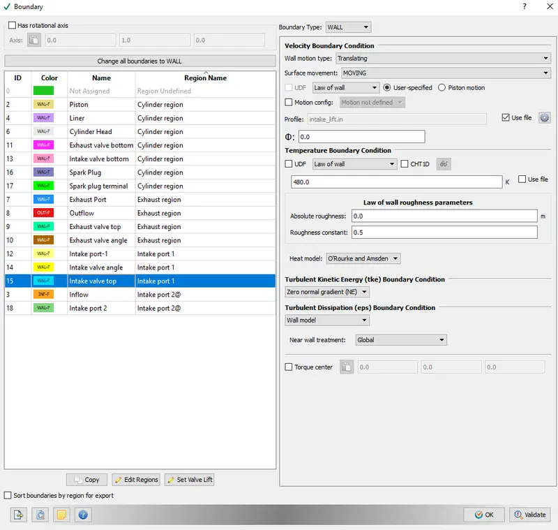
The intake valve motion file was imported.

4.15. Inflow

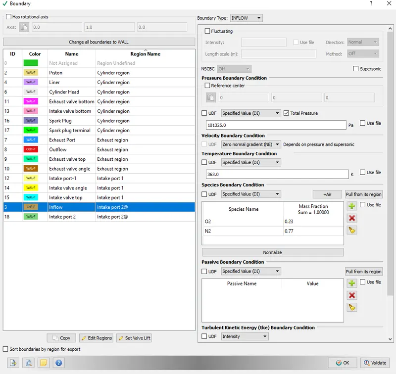
4.16. Intake port 2

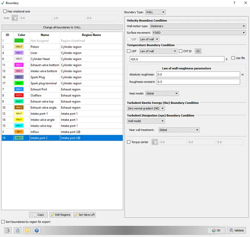
5. Region Initialization

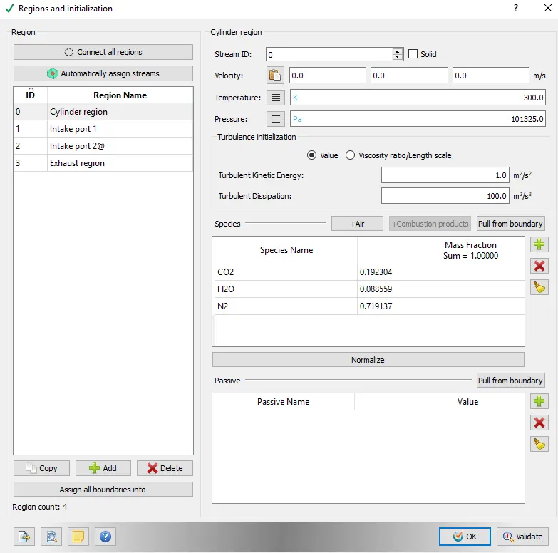
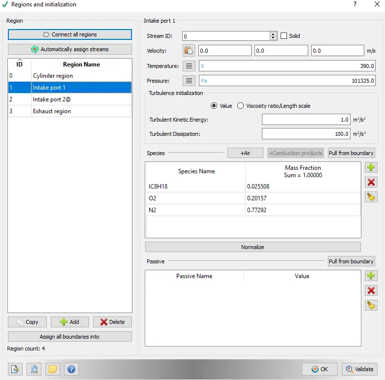
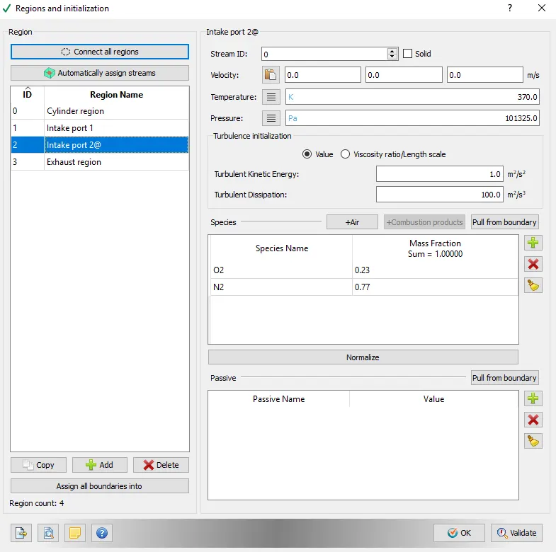
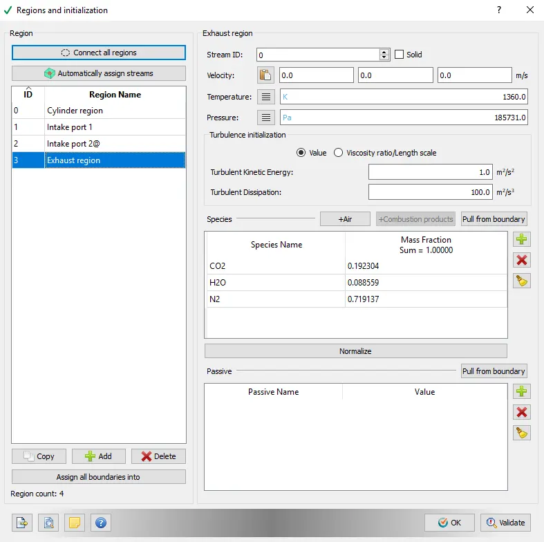
Region Initialization is important to help us dividing complex geometries into separate entities according to their function, and helps us provide important physical properties such as velocity, temperature, pressure, and species mass fraction, which helps us to achieve convergence quickly.

5.1. Cylinder region

5.2. Intake Port 1

5.3. Intake Port 2

5.4. Exhaust region

6. Events

Events help us to decide how the interface between any two regions behave. For eg. we can set valve event between cylinder region and exhaust region, and it will create disconnect triangles when the valve is supposed to be closed and remove the discoonect triangles when the valve starts to open.

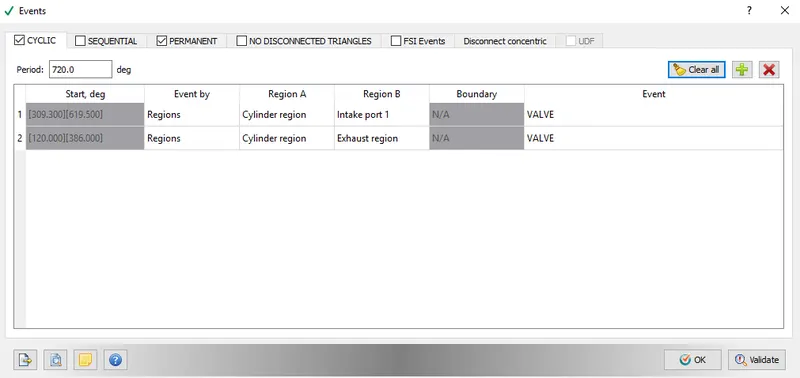
Intake port 1/Exhaust region and Cylinder region interface create disconnect triangles according to the valve profile.

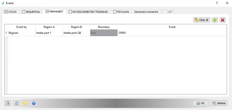
Intake port 1 and Intake port 2 are permanently open.

7. Physical Models

7.1. Spray modeling:

Spray modeling is used to configure nozzles, injectors, boundary injections, injection rate-shapes, set various spray-related constants, and choose from several injection and drop models. Spray modeling is very important to obtain accurate solutions for predictive combustion simulations. Converge has a variety of spray modeling options. In this project, we will be using the O'rouke model for the turbulent dispersion of spray parcels. It also has the option to create collision mesh, and model spray-wall interaction. We have selected the option to form a film on the cylinder wall.

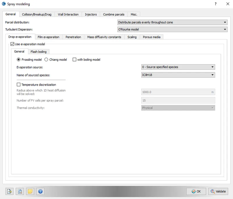
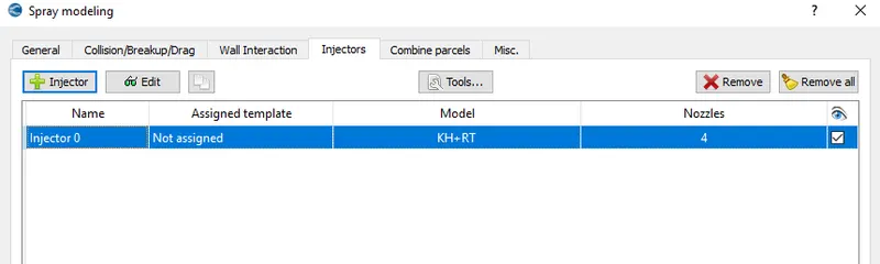
First, we need to create an injector.

We have to specify the injected parcel species and mass fraction.

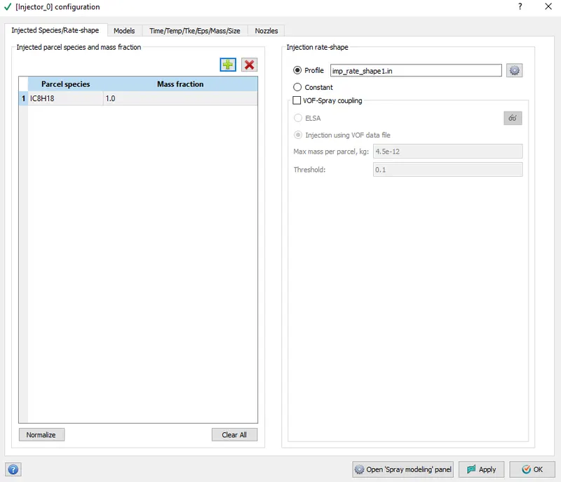
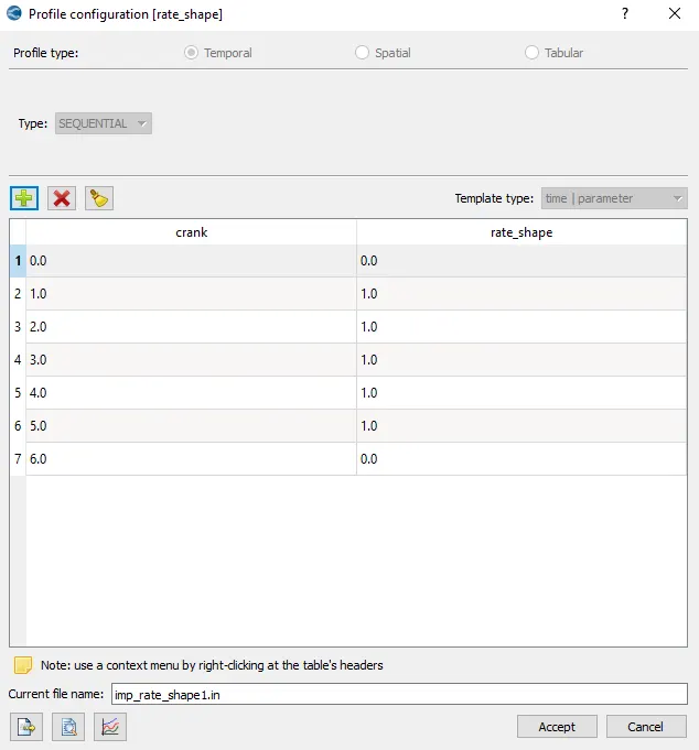
We also have to specify the profile rate shape of the injector.

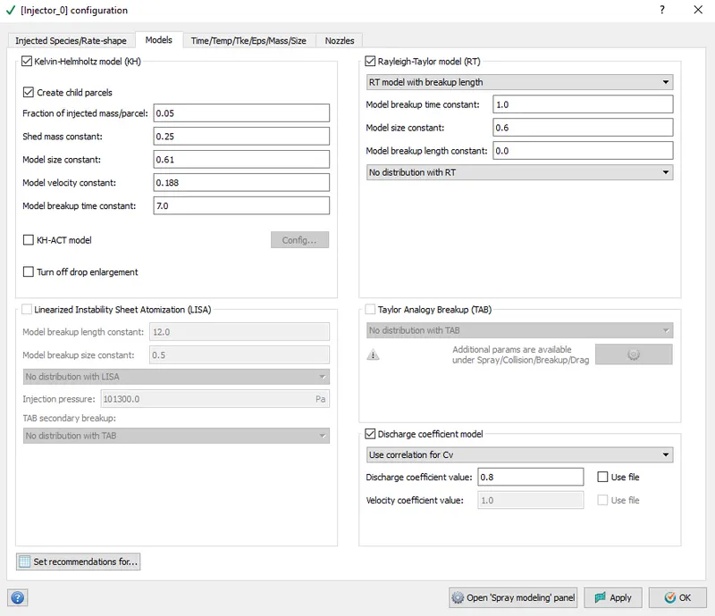
Kelvin-Helmholtz model and Rayleigh-Taylor model is used to model the spray formulation and break-up.

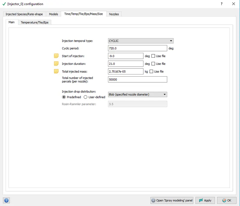
Injection properties:

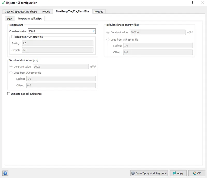
The temperature of the parcels being injected has to be specified.

A total of 4 nozzle injectors were created.

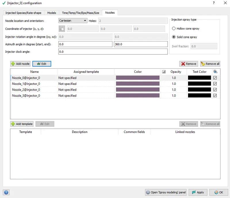
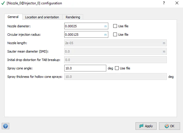
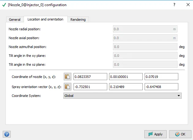
Nozzle properties for the four nozzles were specified.

• Nozzle 0
  • center 0.0823357 0.00100001 0.07019
  • Align Vector -0.732501 0.210489 -0.647408
• Nozzle 1
  • center 0.0823357 -0.00099999 0.07019
  • Align Vector -0.732501 -0.210489 -0.647408
• Nozzle 2
  • center 0.0823357 -0.0004 0.07019
  • Align Vector -0.5 -0.2 -0.647408
• Nozzle 3
  • center 0.0823357 0.0003 0.07019
  • Align Vector -0.5 0.2 -0.647408

All dimensions in m.

7.2. Combustion modeling:

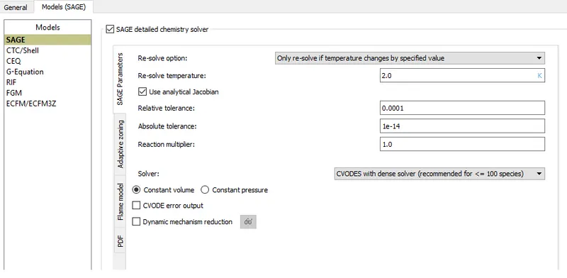
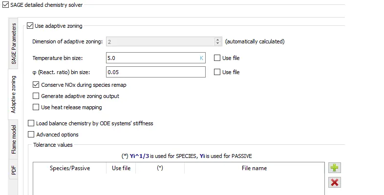
CONVERGE’s SAGE detailed chemistry solver uses local conditions to calculate reaction rates based on the principles of chemical kinetics. This solver is fully coupled to the flow solver, but the chemistry and flow solvers parallelize independently of one another, which speeds up the simulation.

Detailed chemistry modeling can be expensive, and so CONVERGE incorporates numerous acceleration strategies such as adaptive zoning, dynamic mechanism reduction, and stiffness-based load balancing. These techniques, coupled with strategies to speed up species transport, allow you to use more detailed reaction mechanisms to accurately simulate kinetically limited phenomena and emissions. CONVERGE also contains utilities for zero-dimensional ignition delay, mechanism merging and reduction, sensitivity analysis, and one-dimensional laminar flame speed. These utilities enhance the use of detailed chemistry.

I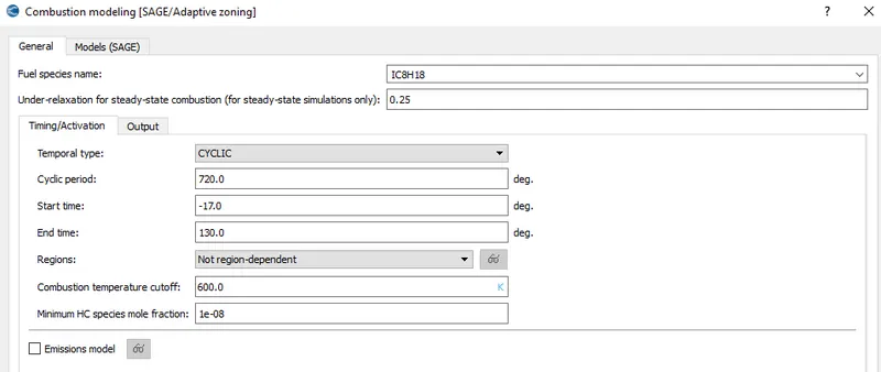

7.3. Turbulence modeling:

8. Grid Control

8.1. Base Grid

8.2. AMR

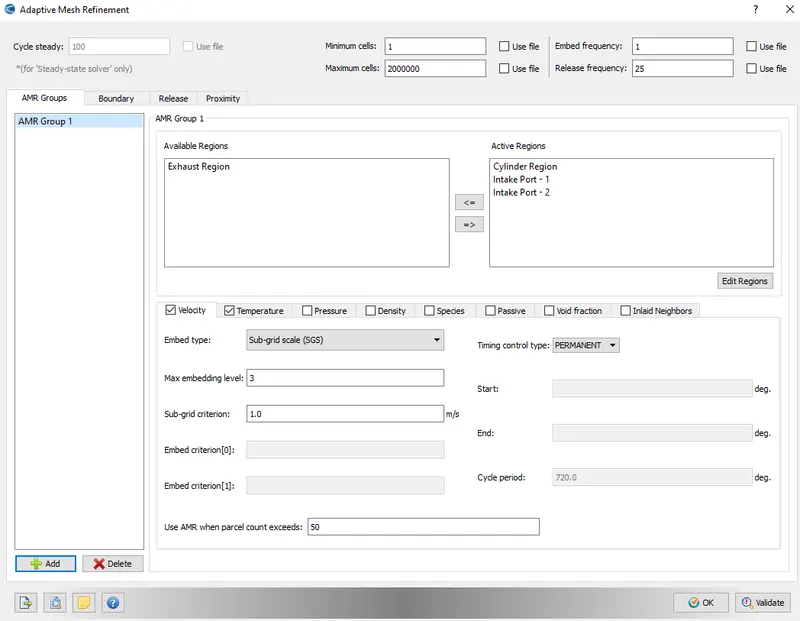
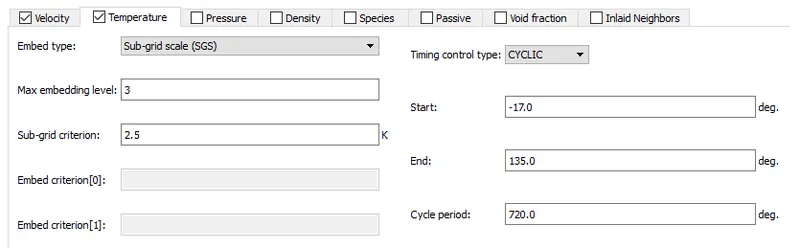
Enable the velocity and Temperature AMR as shown below. AMR stands for Adaptive mesh refinement, it refines the mesh in the critical areas where the gradients of key variables (for ex: velocity, temperature) are very high and these areas require more accuracy for the overall solution to be accurate.

Here the sub-grid criterion is the limit beyond which AMR will be enabled. Max Embedding level is the scale up to which the refinement will be done.

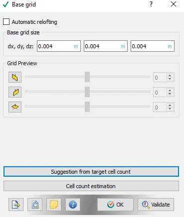
max embedding level of 3 for a mesh size of 4 mm will refine the mesh up to 4/2^3 = 4/8 = 0.5 mm mesh size

8.3. Fixed embedding

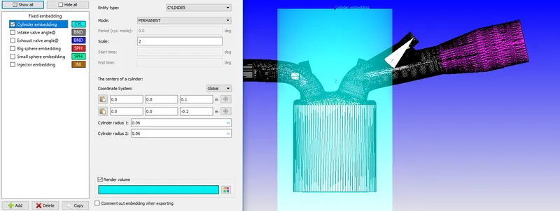
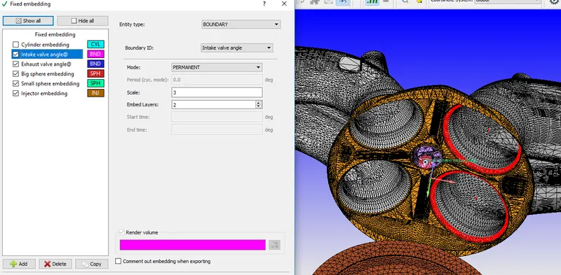
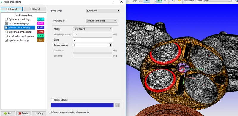
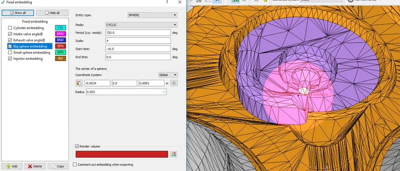
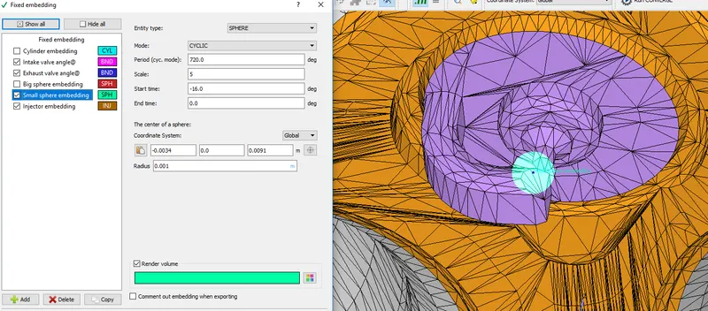
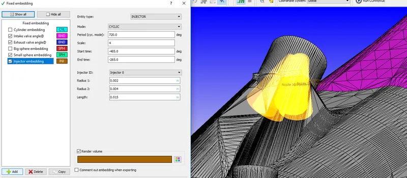
Fixed Embedding is done to refine the mesh size in critical boundaries like the valve angle boundaries, inside the cylinder (where combustion takes place), the region near the spark plug, and the fuel injector.

Scale decides how small the refinement will be according to the formula, refined mesh size = (base grid size/ 2^n); where n is the scale

And, Layers decide in how many steps will the refinement be done; to obtain a refined mesh smoothly.

8.3.1. Cylinder embedding

8.3.2. Intake valve angle

8.3.3. Exhaust valve angle

8.3.4 Big Sphere embedding 

8.3.5 Small Sphere embedding

 

8.3.5 Injector embedding

 

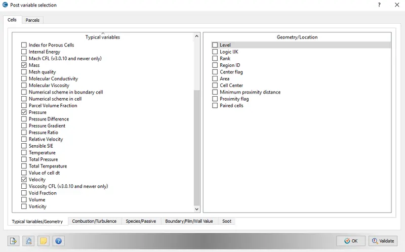
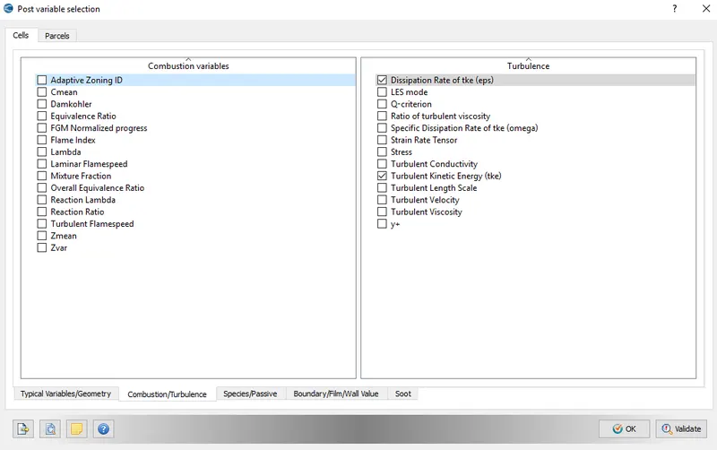
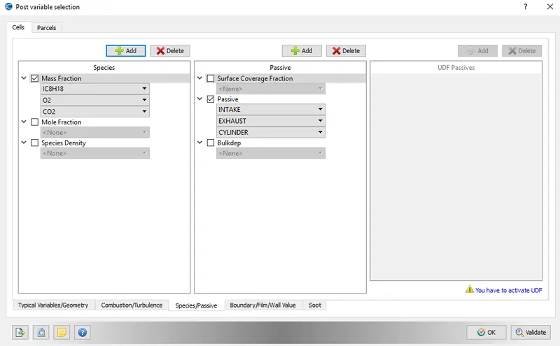
9. Output variables

10. Output files

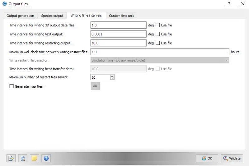
The input files were exported to a file and using Cygwin command line, we used converge-intelmpi solver to run a parallel simulation with 4 processors.

Using the post-processing tools, the output files obtained were converted into Paraview VTK in-line binary format file type which can be then opened by ParaView.

Importance of Ring triangles:

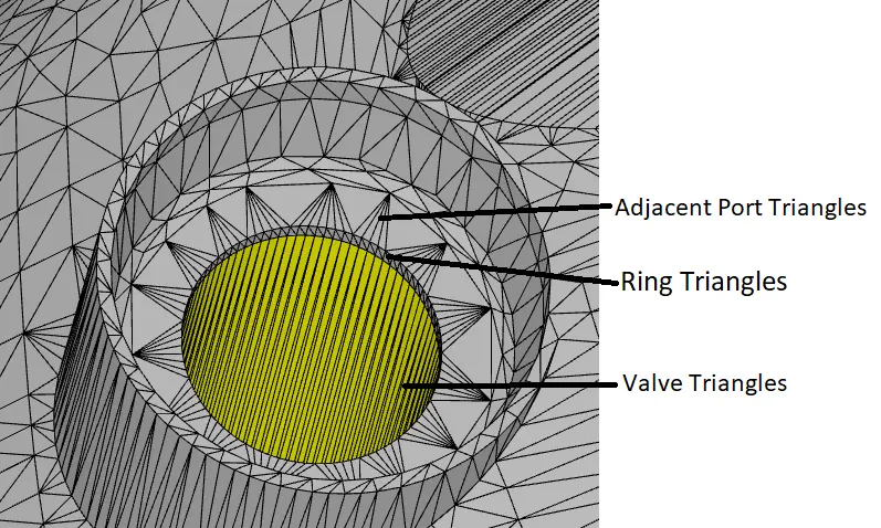
When the valve triangles move up and down in a periodic motion, the very adjacent port triangles (of a different boundary) get warped if the ring triangles are not created.

The ring triangles are created so that when the valve triangles move up and down periodically, the ring triangles get stretched without changing its shape.

Simulation Results

Pressure Plot

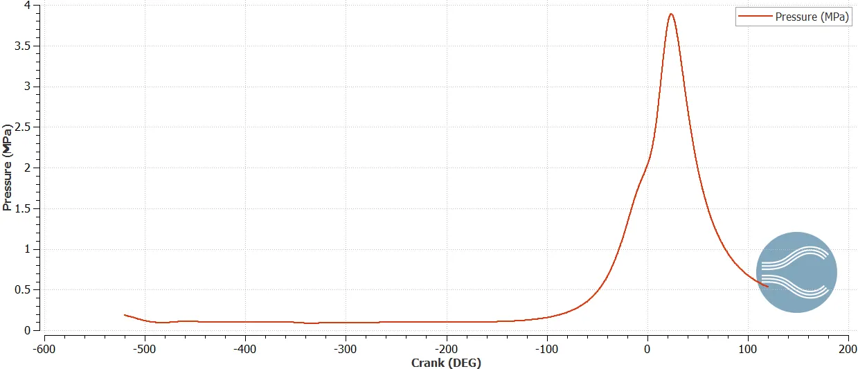
The pressure starts increasing from -160 degrees (BDC) due to compression. At -16 degrees (TDC) the igniter starts the combustion process and there is a steep rise in pressure till about 23 degrees, this pressure rise is due to the combustion process. The maximum pressure reached is 3.88 MPa @ 23.64 degrees.

Temperature Plot

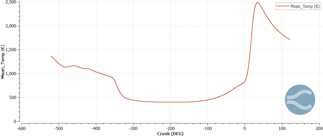
The above plot shows the mean temperature inside the cylinder at different crank angles. The maximum temperature is 2483 K which occurs at 33 degrees (right after combustion).

Volume Plot

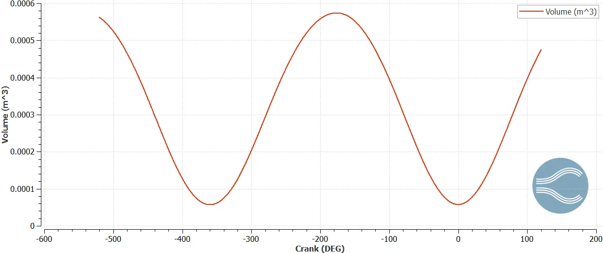
The Volume keeps changing due to the piston movement, Minimum volume at TDC, and Maximum volume at BDC.

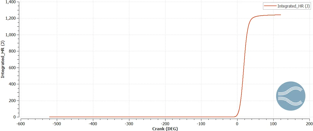
Integrated Heat Release

Fuel Spray

Drops

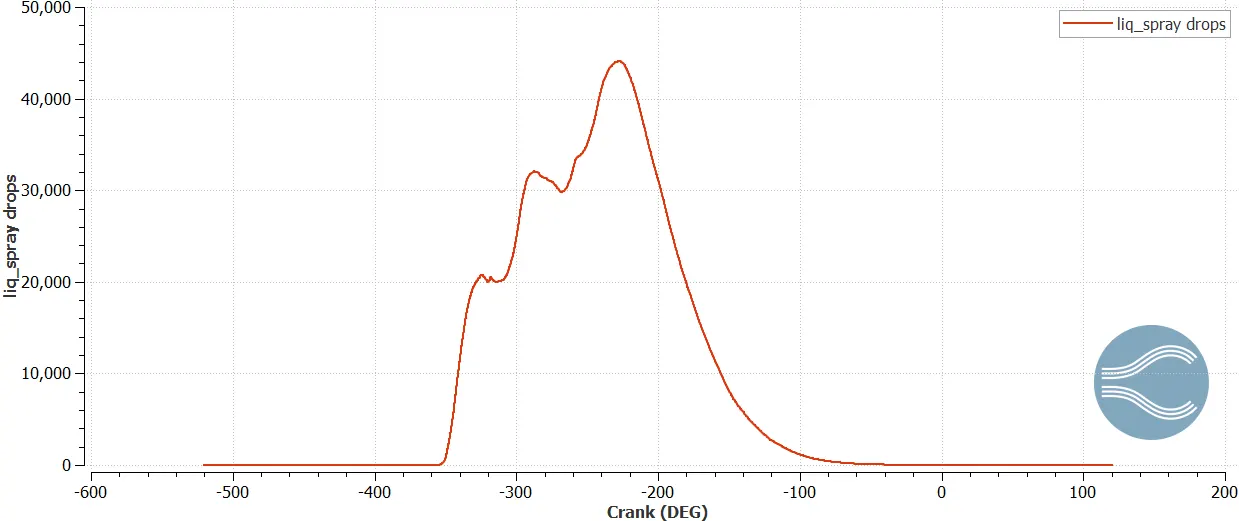
The above plot shows the number of fuel drops at different crank angles.

Emissions Plots

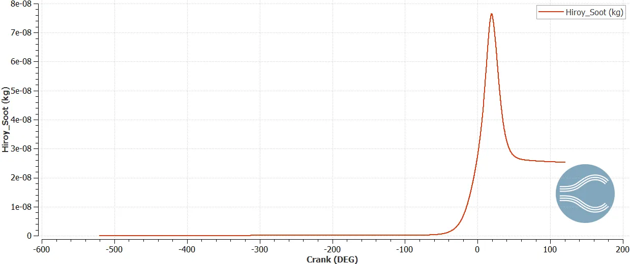
1. Soot Formation

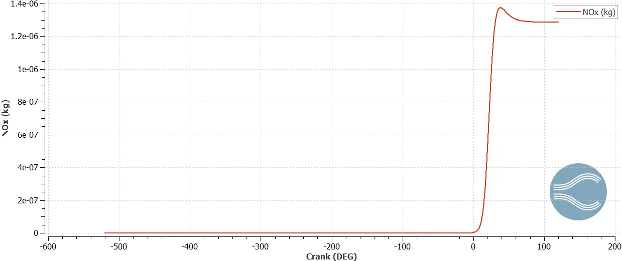
2. NOx Formation

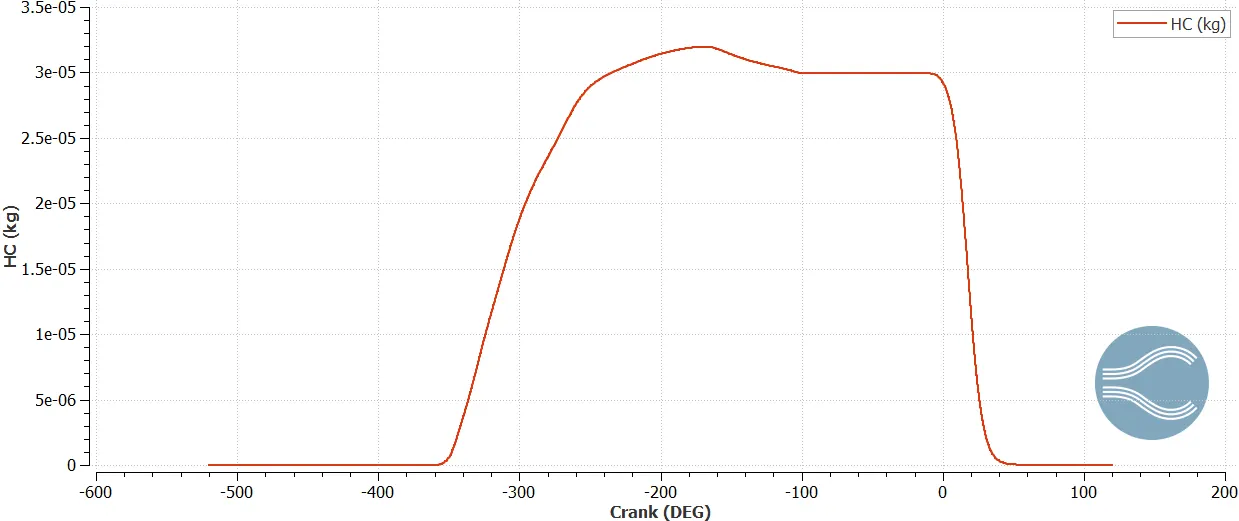
3. Hydro-Carbons

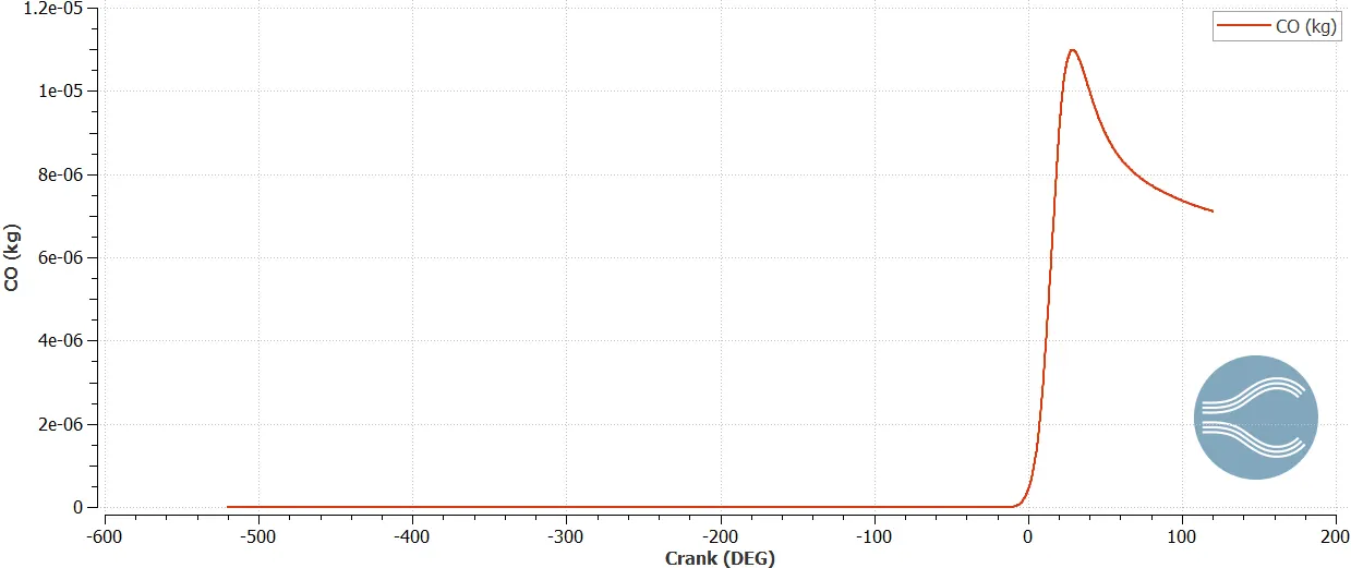
4. CO formation

5. CO2 Formation

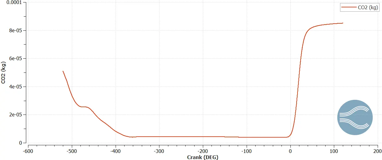
From the above plots:

Max Soot formation: 7.63e-8 kg

Max NOx formation: 1.37e-6 kg

Max HC formation: 3.1e-5 kg

Max CO formation: 1.09e-5 kg

Max CO2 formation: 8.5e-5 kg

Animation

The below animation shows how the Lagrangian fluid parcels move from the intake port to the cylinder and how the larger fuel parcels break down into smaller parcels and then vaporizes.

Also, we can observe the change in temperature contour region by region as the cycle progresses.

Dynamic mesh generation:

We can observe the embeddings are created according to our inputs.

Questions:

1. What is the compression ratio of this engine?

Volume vs Crank Angle Plot

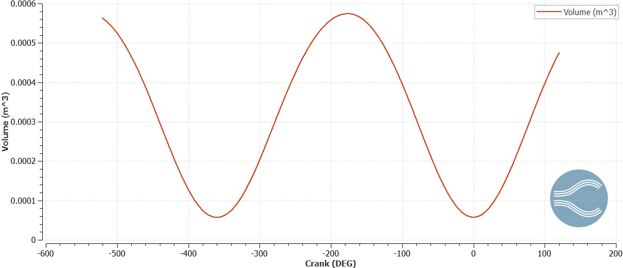
Here the maximum volume is = 0.0005738 `m^3` and the minimum volume is =  5.7032 e-5 `m^3`

Compression Ratio = `("maximum volume")/("minimum volume")` = 0.0005738 / 5.7032e-5 = 10.06

2. Why do we need a wall heat transfer model? Why can't we predict the wall temperature from the CFD simulation?

We have used a wall heat transfer model because we are interested in the fluid flow and heat transfer occurring in the fluid domain and are not solving for the heat transfer through the solid cylinder, since then it will become a CHT simulation which will be computationally expensive. Hence by using wall heat transfer models we can speed up the process.

3. Calculate the combustion efficiency of the engine

Combustion efficiency = Actual Heat released / Heat released when fuel is completely burned

We can calculate the actual heat released from the fuel using the Integrated Heat Released Line plot.

Actual Heat Released from fuel = 1241.16 Joules

Injected Fuel Mass = 3e-5 kg

Calorific Value of IC8H18 = 44.65 MJ/kg

Heat Input = 44.65 * 10^6 * 3*10^-5 = 1339.5 Joules

So, Combustion efficiency = (1241.16 / 1339.5) *100 = 92.65 %

4. Use the engine performance calculator, to determine the power and torque for this engine.

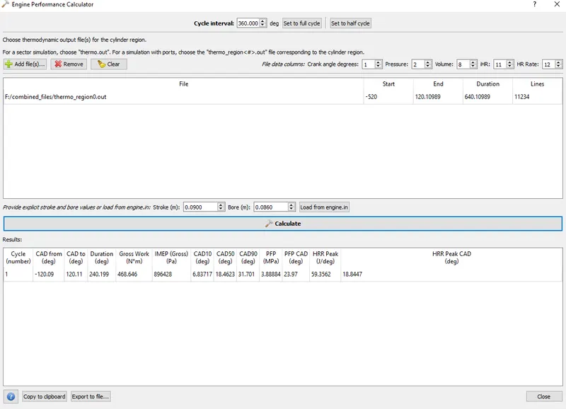
Power = Work per unit time

work done from -120.09 to 120.11 degrees is 468.646 N.m (i.e. 240.2 degrees)

RPM = 3000

Converting RPM to RPS

RPS = 3000/60 = 50

Degrees per second = RPS*360 = 50*360 = 18000 degrees/second

Time for the crank to rotate by 720 degrees = 720 / Degrees per second = 720 / 18000 = 0.04 seconds

So, Power = work done / unit time = 468.646 / 0.04 Watts = 11.716 kW

We know, Power = 2*pi*N*T/60

Torque = (P*60,000)/(2*pi*N) = (11.716*60*1000)/(2*pi*3000) = 37.27 N-m

5. What is the significance of ca10, ca50, and ca90?

CA10 is the Crank angle rotation from the spark till the fuel is burned 10%. It is useful in finding the ignition delay of the engine. The calculated value for the PFI engine is 6.837 degrees.

CA50 is the Crank angle rotation from the spark till the fuel is burned 50%. CA50 indicates the flame speed, high CA50 indicates low flame speed, and vise versa. If flame speed is low, the combustion process gets delayed and which causes a drop in engine efficiency. The calculated value for the PFI engine is 18.46 degrees.

CA90 is the Crank angle rotation from the spark till the fuel is burned 90%. A lower CA90 value indicates faster combustion and high peak pressures and temperatures. Higher pressure gives higher MEP and efficiency. Higher temperature gives more NOx production. The calculated value for the PFI engine is 31.701 degrees.

 Conclusion:

Full-Hydrodynamic simulation of a Port fuel Injected engine was conducted successfully depicting the appropriate motions of valve and piston respectively and the combustion reactions and spray modeling.