Channel-flow simulation using Converge CFD
Aim - To simulate flow through a channel for 3 different mesh sizes using Converge CFD software.
Introduction and Theory - Flows completely bounded by solid surfaces are called internal flows which include flows through pipes (Round cross-section), ducts (Not Round cross-section), nozzles, diffusers. The basic principles involved are independent of the cross-sectional shape, although the details of the flow may be dependent on it. The flow regime (laminar or transition or turbulent) of internal flows is primarily a function of the Reynolds number (inertial force/viscous force).In pipes, Reynolds number below 2000 is laminar, between 2000 and 4000 is transition flow, above 4000 is turbulent flow.
In pipe flow, the pressure gradient along the pipe is the main driving force.
One important concept in pipe flows, is that of the boundary layer. A boundary layer is the layer of fluid in the immediate vicinity of a bounding surface where the effects of viscosity are significant.
Boundary layers may be either laminar (layered), or turbulent (disordered) depending on the value of the Reynolds number. For lower Reynolds numbers, the boundary layer is laminar, and the streamwise velocity changes uniformly as one moves away from the wall. For higher Reynolds numbers, the boundary layer is turbulent, and the streamwise velocity is characterized by unsteady (changing with time) swirling flows inside the boundary layer. The external flow reacts to the edge of the boundary layer, just as it would to the physical surface of an object. So the boundary layer gives any object an "effective" shape which is usually slightly different from the physical shape. The boundary layer may lift off or "separate" from the body and create an effective shape much different from the physical shape. This happens because the flow in the boundary has very-low energy (relative to the free stream) and is more easily driven by changes in pressure.
Pre-processing:
Step 1: Creating Geometry
A box geometry is created.
Center: 0.05 in +ve x-direction
Size in meters: 0.1 - x-axis, 0.01 - y-axis, 0.01 - z-axis
The following geometry was created:
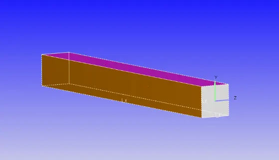
Firstly, make sure the normal to the faces are facing inside towards the fluid domain. If not, under transform, go to normal and select propagate changes from a single triangle. This option will make sure all the normals are facing inwards.Then, appropriate boundaries need to be created and flagged. Boundaries can be identified from the color code provided next to the boundary name.
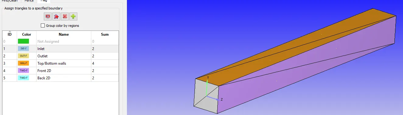
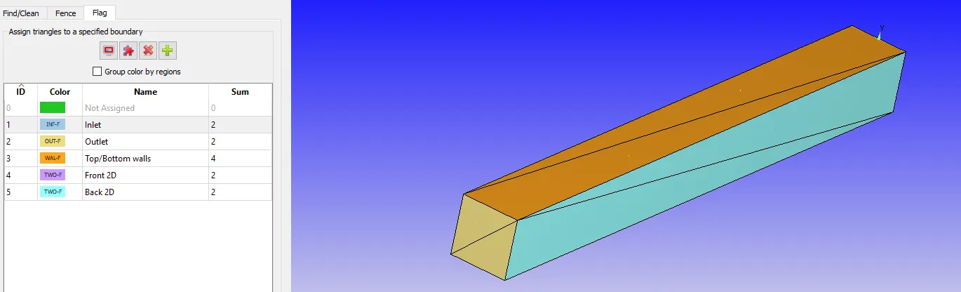
Step 2: Case Setup
Application Type: Time-based
Materials:
1. Gas simulation
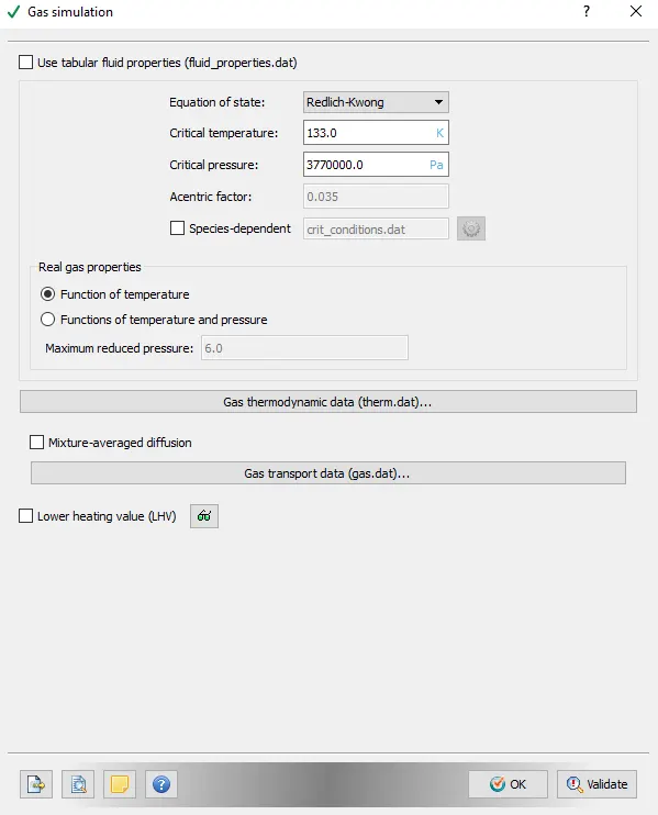
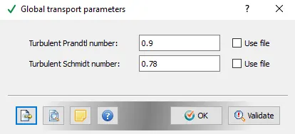
2. Global transport parameters
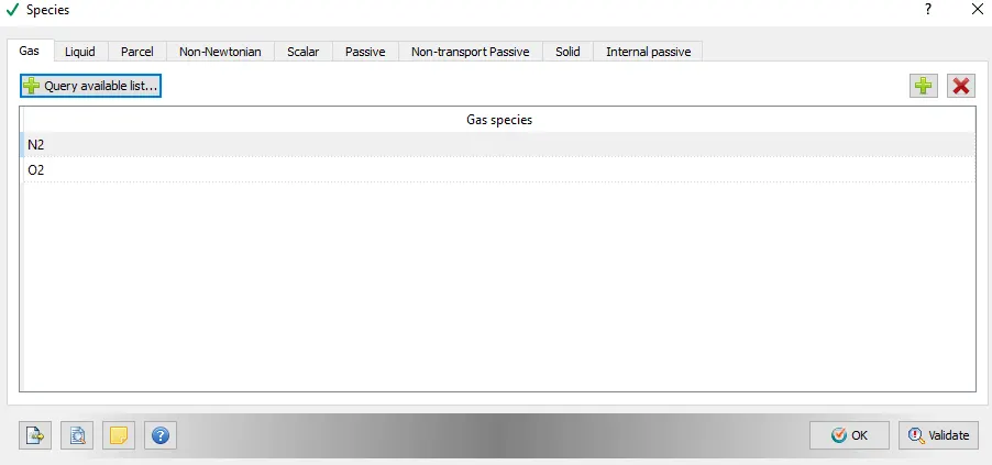
3. Species
Simulation parameters:
1. Run parameters:
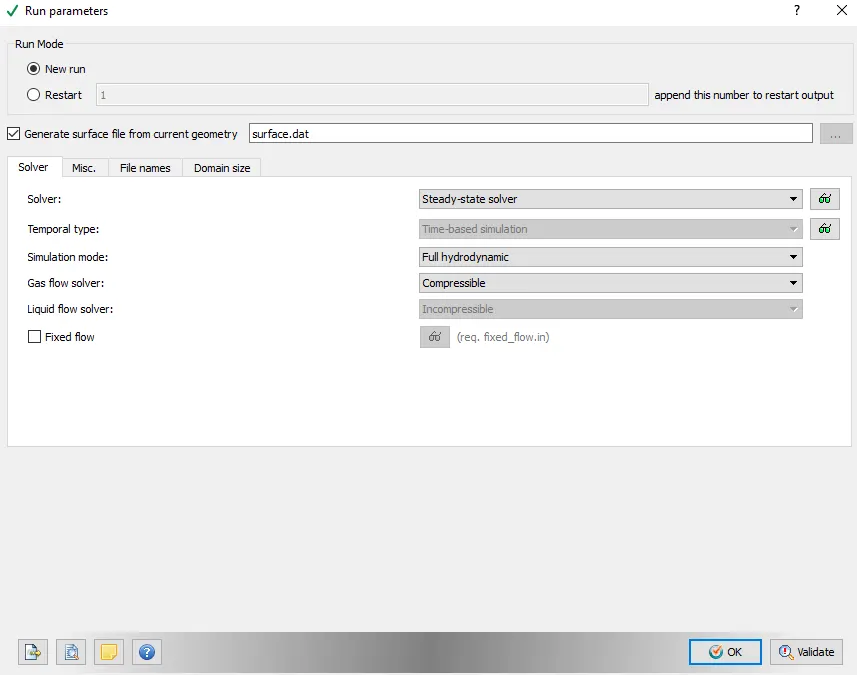
Switch off shared memory.
1.1. Steady-state monitor
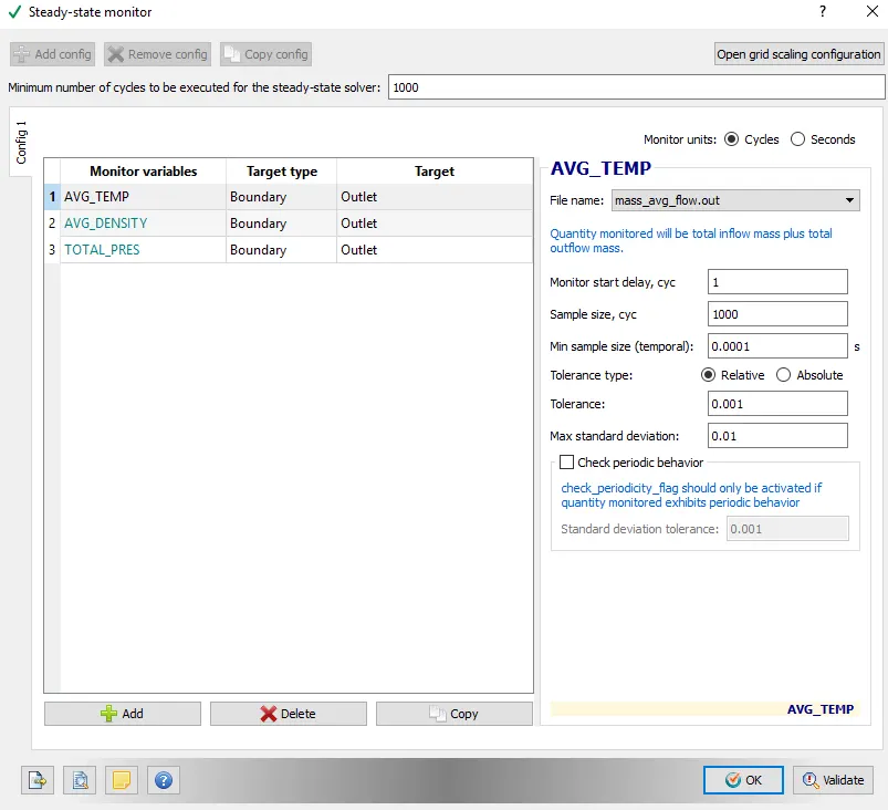
1.2. Simulation time parameters
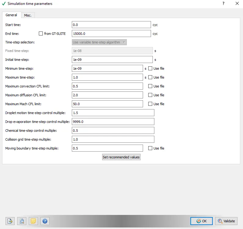
1.3. Solver parameters
Solver Scheme: PISO
Solver Type: Density-based
Maximum Convection CFL limit = 0.5
Pressure Pre-conditioner = None
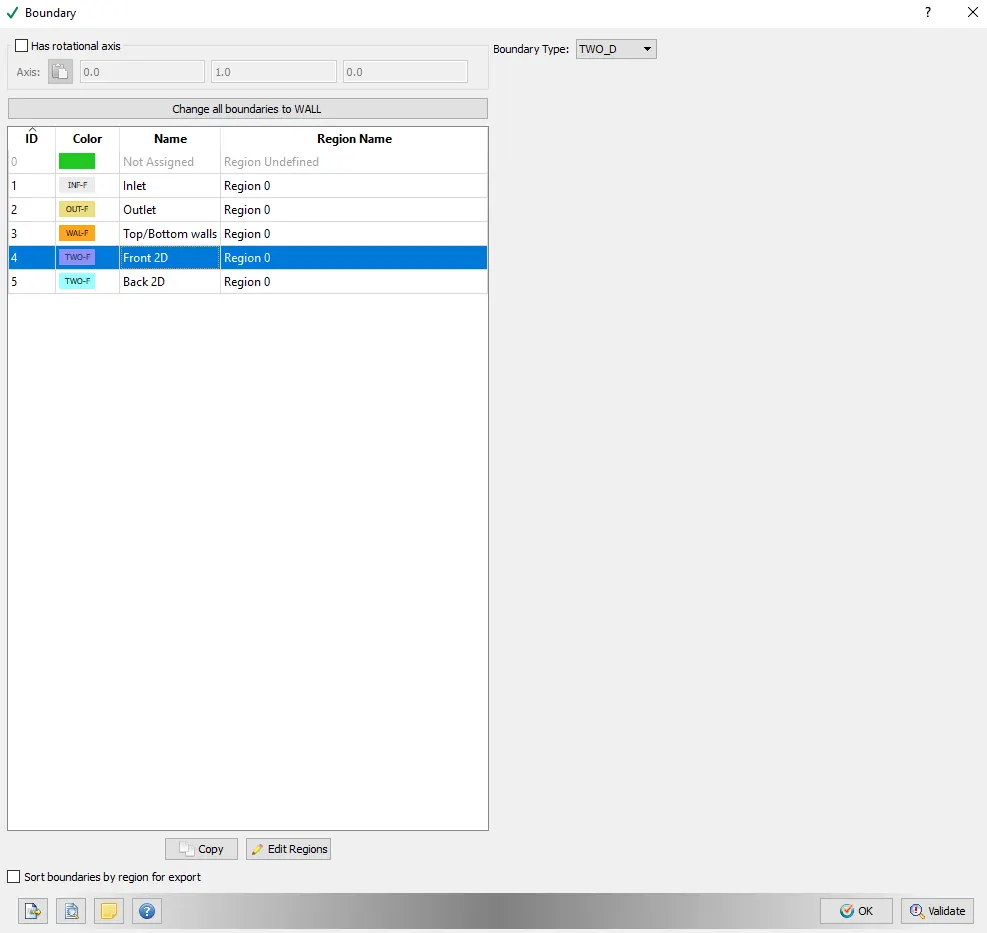
Boundary Conditions:
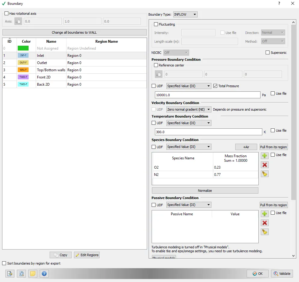
Inlet:
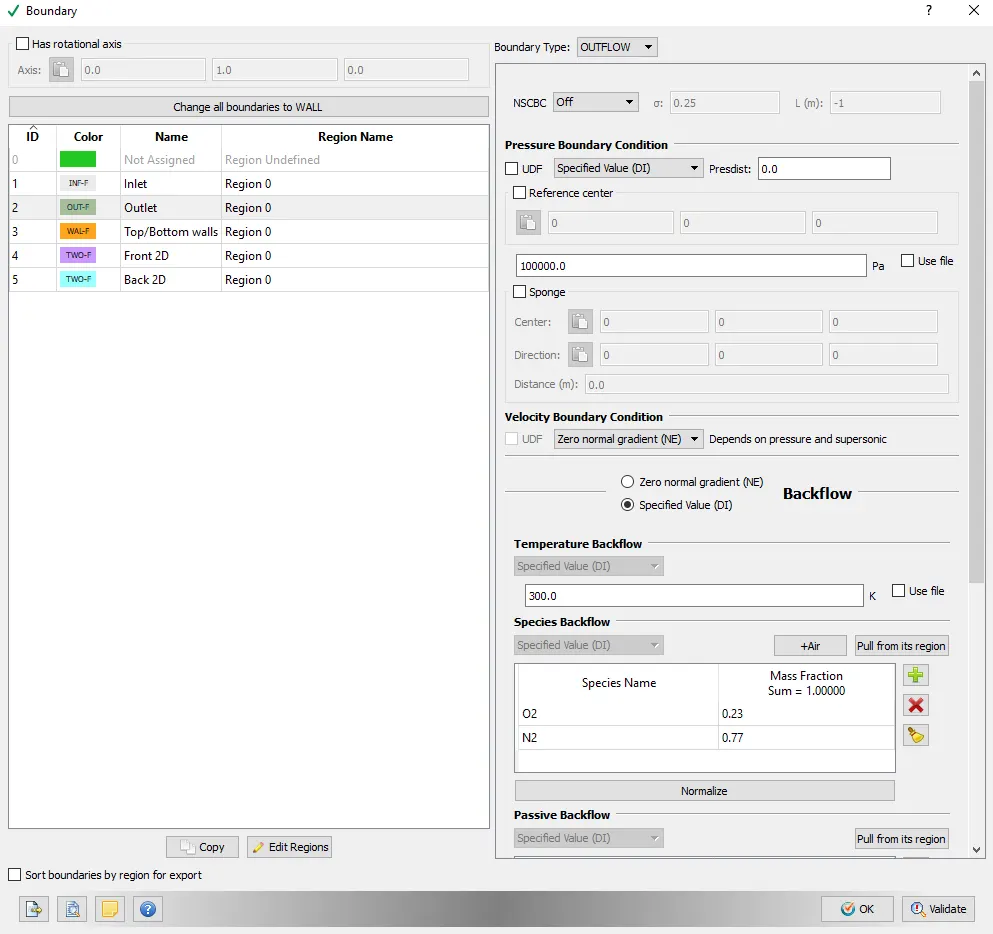
Outlet:
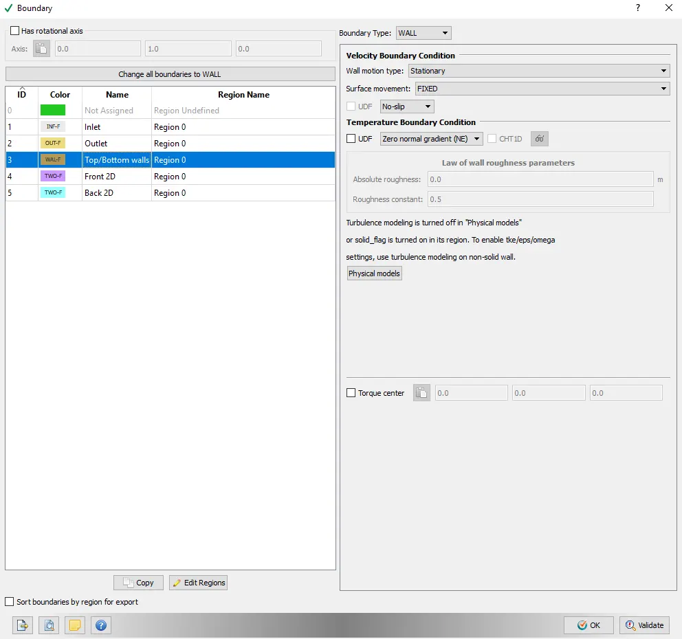
Top/Bottom Walls:
Front 2D and Back 2D:
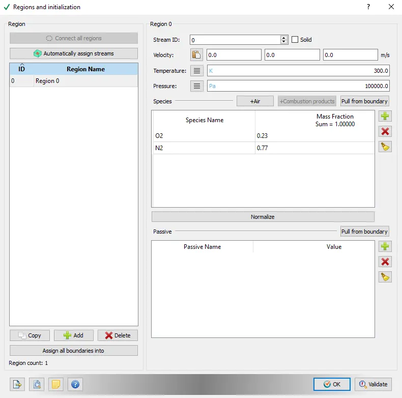
Regions and Initialization:
Grid control:
1. Base Grid
1.1 Mesh 1: dx=3e-4 m, dy=3e-4 m, dz=3e-4 m

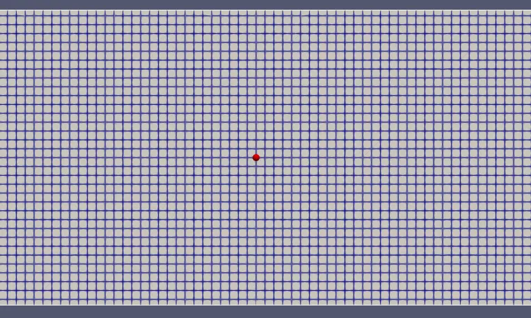
1.2 Mesh 2: dx=2e-4 m, dy=2e-4 m, dz=2e-4 m
Far view:

Close-up view:
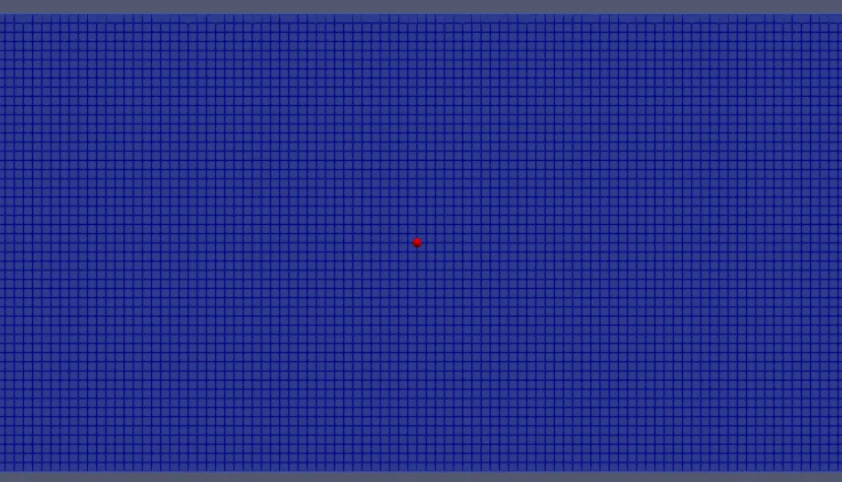
1.3 Mesh 3: dx=1e-4 m, dy=1e-4 m, dz=1e-4 m

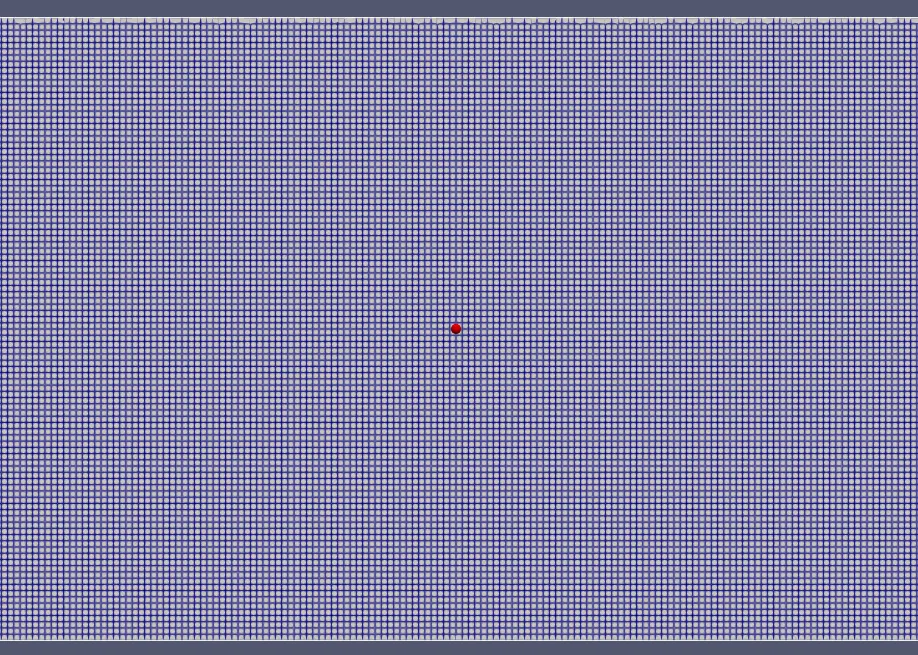
Post-Processing:
1. Post variable selection - Pressure, Temperature, Velocity
2. Output files -
The time interval for writing 3D output data files: 100
The time interval for writing restarting output: 100
Maximum restart files saved: 3
Results:
Case 1:
1. Velocity contour:
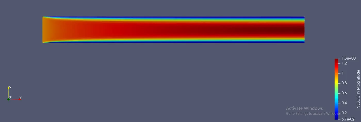
The velocity contour depicts the formation of the boundary layer.
2. Pressure contour:
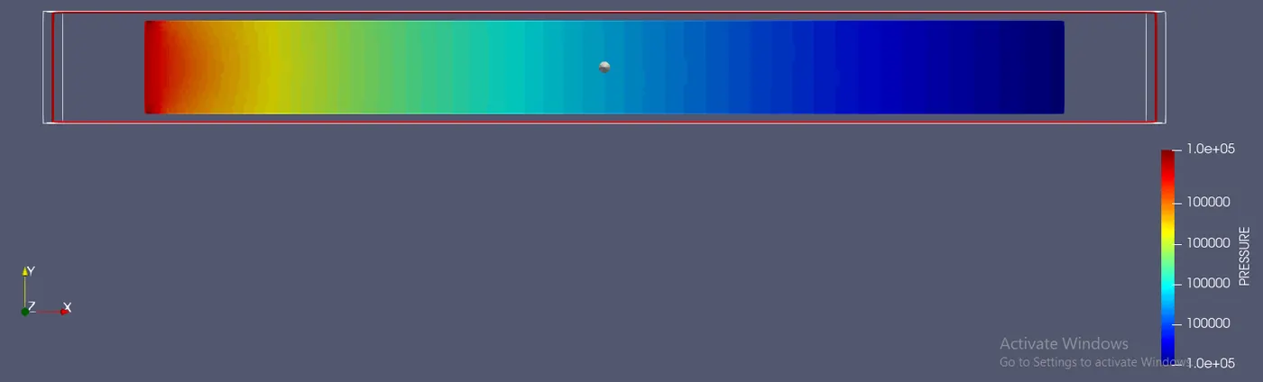
Pressure contour is being formed accurately according to the boundary conditions.
3. Velocity plot:
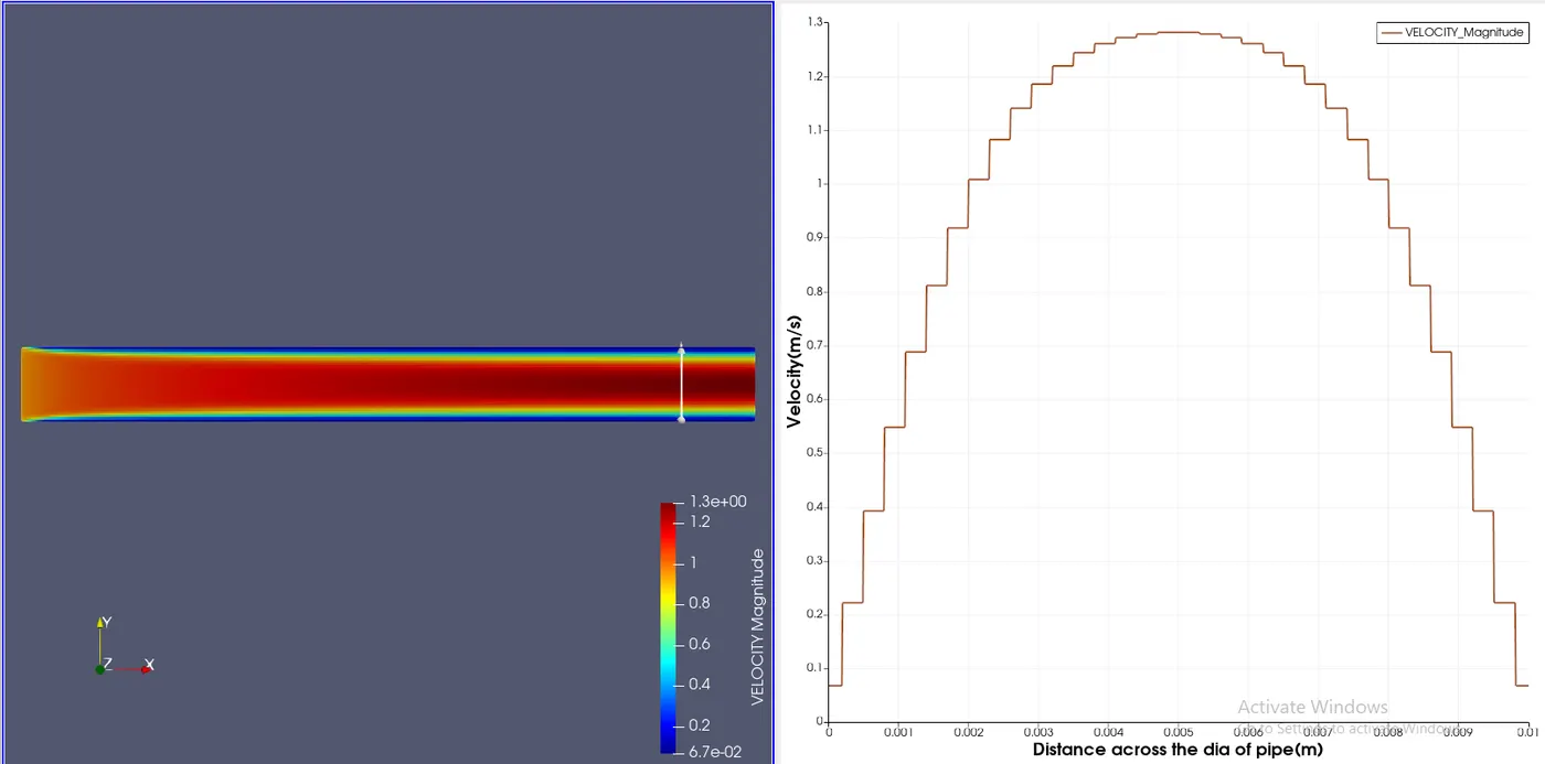
Velocity plot on a vertical line at x=0.09m (near the exit of the channel). The peak velocity near the center of the channel is 1.28159 m/s. The plot values adhere to the principle of boundary layer theory.
4. Pressure plot:
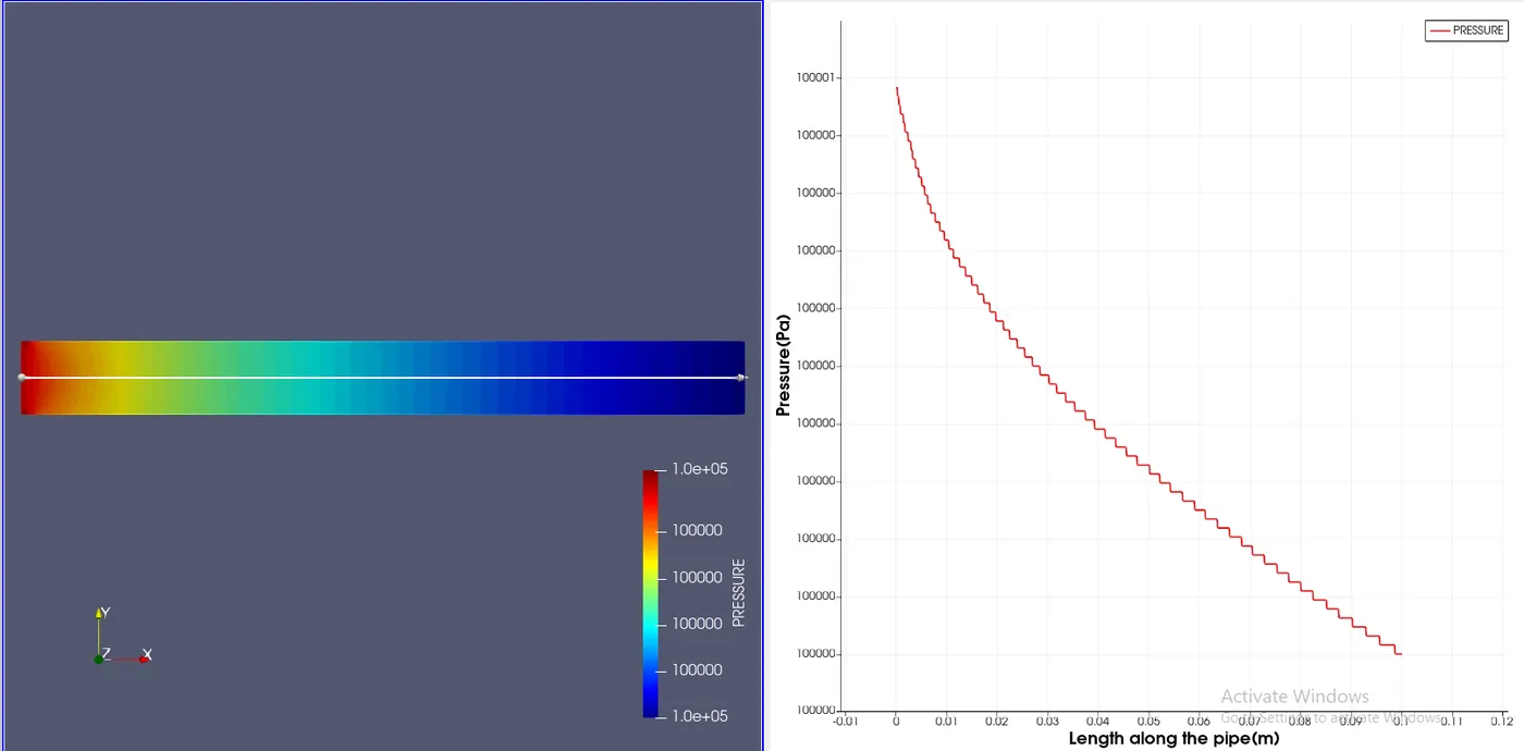
The pressure is constantly decreasing along the pipe as expected according to the boundary conditions given.
5. Mass flow rate:
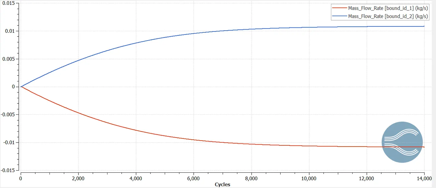
The mass flow rate is -0.0108252 m/s for the inlet and 0.0108251 m/s for the outlet. (The sign indicates if the flow is inside the channel or outside the channel)[Bound_Id_1 and Bound_Id_2 stands for the inlet and outlet boundary respectively]
6. Cell count:
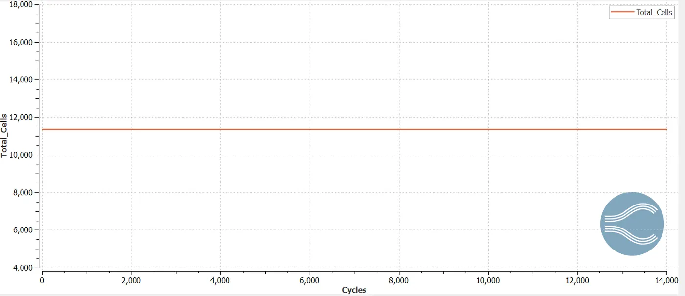
The cell count for the first mesh is 11,356.
Case 2:
1. Velocity contour:
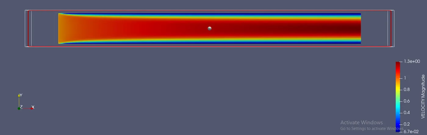
The velocity contour depicts the formation of the boundary layer.
2. Pressure contour:
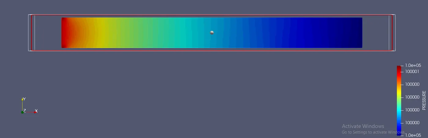
Pressure contour is being formed accurately according to the boundary conditions.
3. Velocity plot :
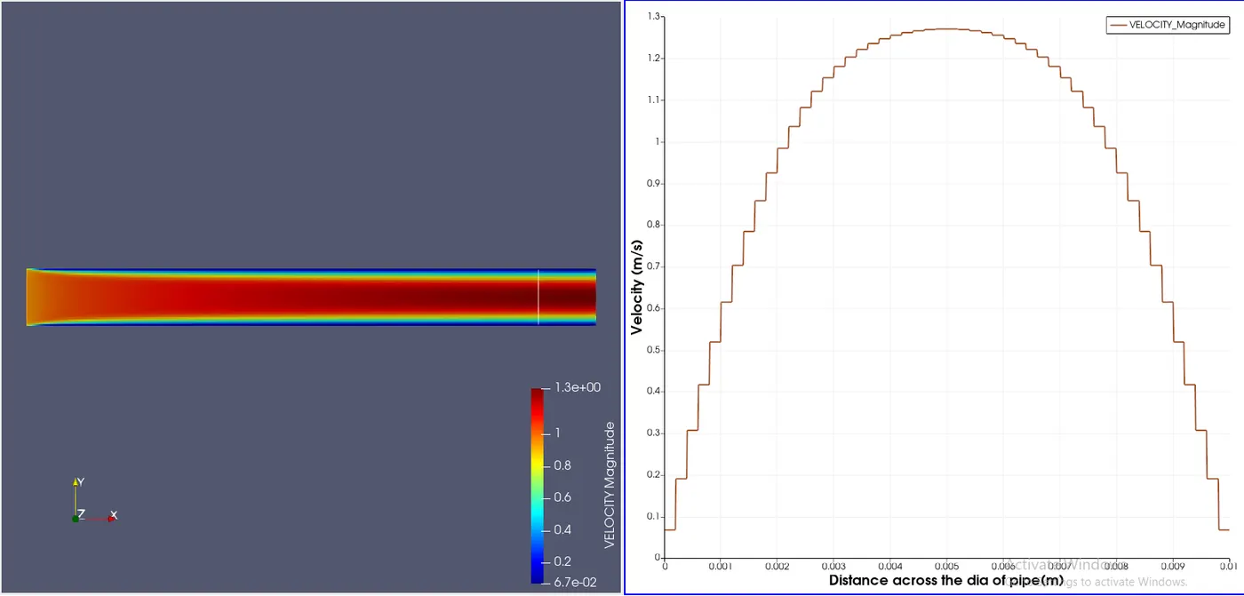
Velocity plot on a vertical line at x=0.09m (near the exit of the channel). The peak velocity near the center of the channel is 1.27049 m/s. The plot values adhere to the principle of boundary layer theory.
4. Pressure plot:
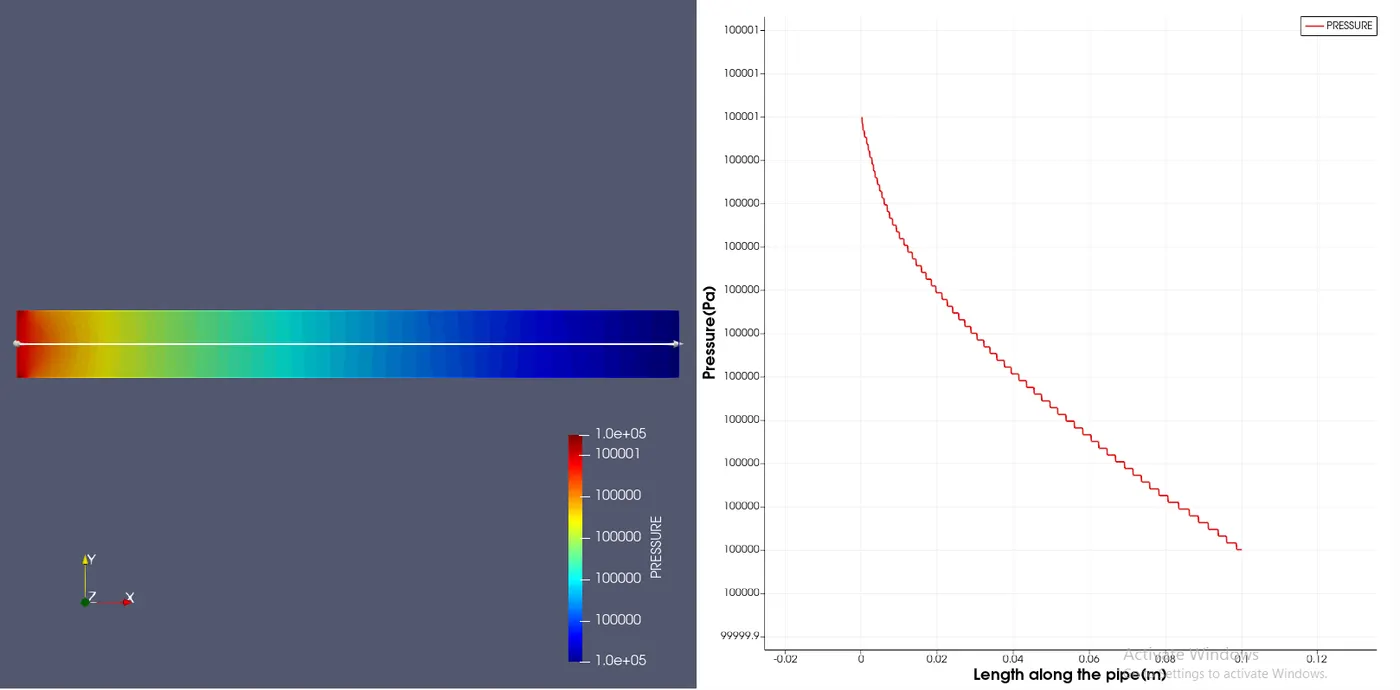
The pressure is constantly decreasing along the pipe as expected according to the boundary conditions given.
5. Mass flow rate:
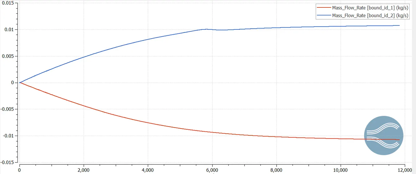
The mass flow rate is -0.0107176 m/s for the inlet and 0.0107124 m/s for the outlet. (The sign indicates if the flow is inside the channel or outside the channel)[Bound_Id_1 and Bound_Id_2 stands for the inlet and outlet boundary respectively]
6. Cell count:
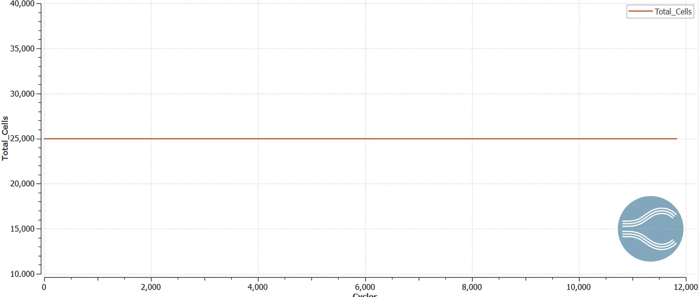
The cell count for the second mesh is 25,000.
Case 3:
1. Velocity contour:
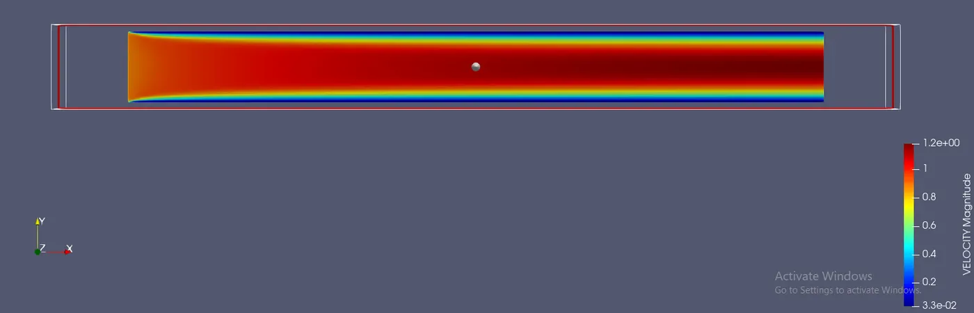
The velocity contour depicts the formation of the boundary layer.
2. Pressure contour:
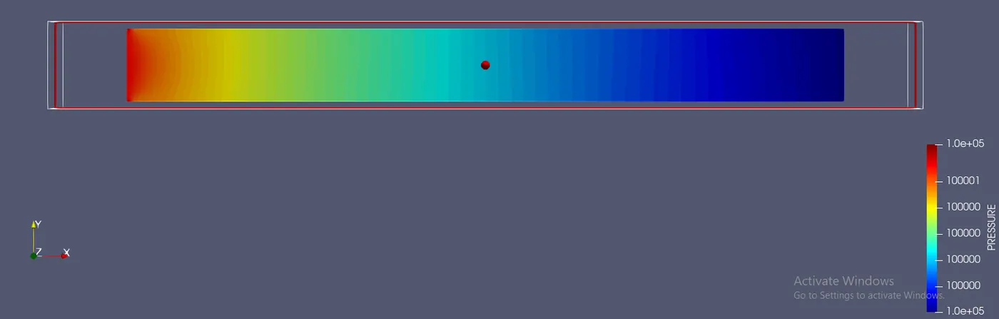
The pressure is constantly decreasing along the pipe as expected according to the boundary conditions given.
3. Velocity plot:
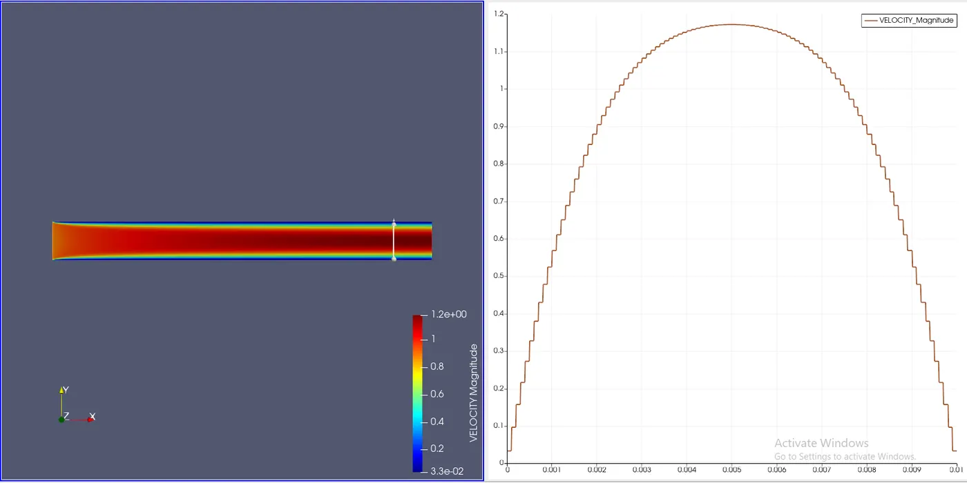
Velocity plot on a vertical line at x=0.09m (near the exit of the channel). The peak velocity near the center of the channel is 1.17224 m/s. The plot values adhere to the principle of boundary layer theory.
4. Pressure plot:
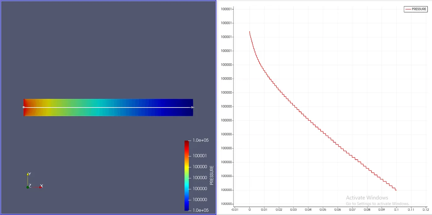
The pressure is constantly decreasing along the pipe as expected according to the boundary conditions given.
5. Mass flow rate:
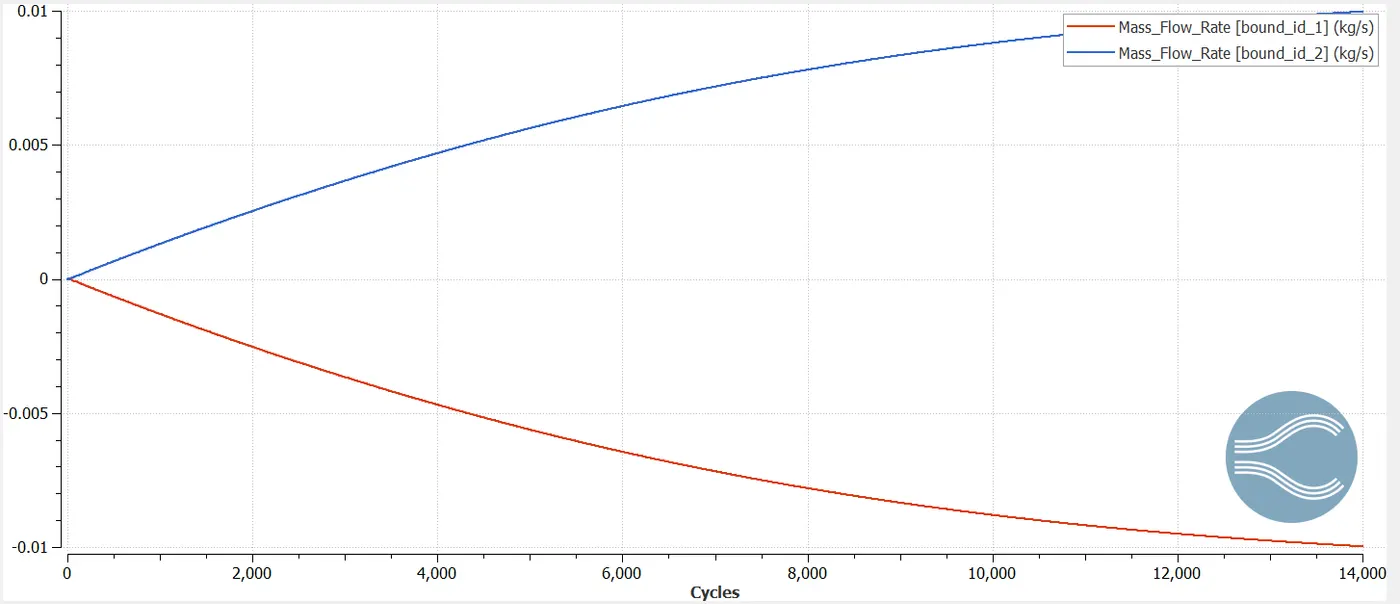
The mass flow rate is -0.00997052 m/s for the inlet and 0.00997051 m/s for the outlet. (The sign indicates if the flow is inside the channel or outside the channel)[Bound_Id_1 and Bound_Id_2 stands for the inlet and outlet boundary respectively]
6. Cell count:
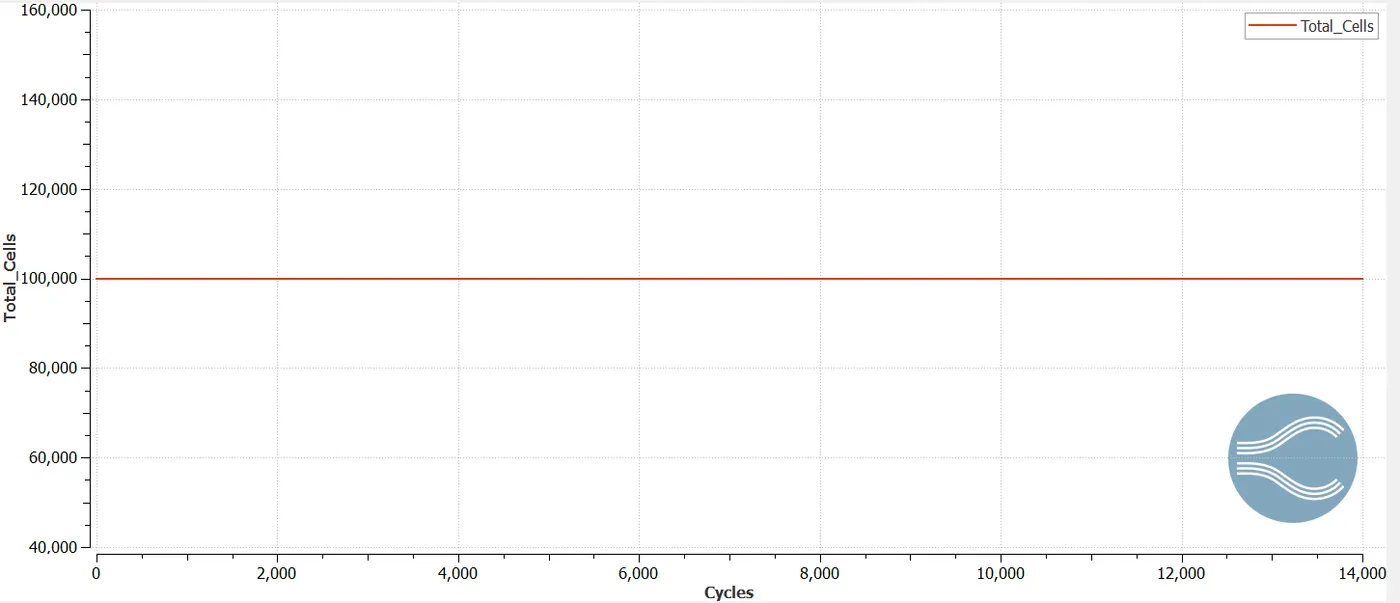
The cell count for the third mesh is 100,000.
Velocity Animation:
From the velocity animation, we can clearly see the velocity development inside the channel. In the starting, the entire domain was blue(i.e zero velocity), but as the iterations were calculated, in the center of the channel the velocity slowly starts to increase, and it keeps on increasing until a max value of velocity is achieved at the pipe center. At the pipe walls, no-slip condition was applied, hence we can observe the formation of a parabolic profile boundary layer, which agrees with the physical experiments.
Pressure Animation:
From, the pressure animation we can see a smooth decrement in pressure along the channel which is in keeping with the physical experiments and boundary conditions.
Conclusion:
1. The pressure is the driving force for the flow through the channel hence pressure keeps on decreasing which can be confirmed from pressure contours.
2. Velocity contours depict the formation of no-slip condition at the wall. This helps in the formation of parabolic shaped boundary layers.
3. The plots are in the form of steps because of the mesh size. The finer the mesh, smoother will be the curve.
4. The mass-flow rate graphs confirm the conservation of mass. It is observed that the mass-flow rate value decreases by a very small amount as the mesh becomes finer.
5. The peak velocity value also drops as the mesh becomes finer.