Backward Facing Step Simulation using Converge CFD
Aim: To simulate flow over a backward-facing step for different mesh sizes.
Introduction and Theory: Backward-Facing Step (BFS) flow is a representative model for separation flows, which can be widely seen in aerodynamic flows (airfoil, spoiler, high attack angle process), engine flows, condensers, vehicles (cars, boat), heat transfer systems, and even the flow around buildings, etc. The flow separation after a simple stage will introduce separation bubble formation, evolution, and re-attachment process, which is dependent on the BFS geometric design, the inlet and outlet conditions, turbulent intensity, as well as heat transfer conditions. In the past decades, it has been widely studied by various theoretical, experimental, and numerical methods.
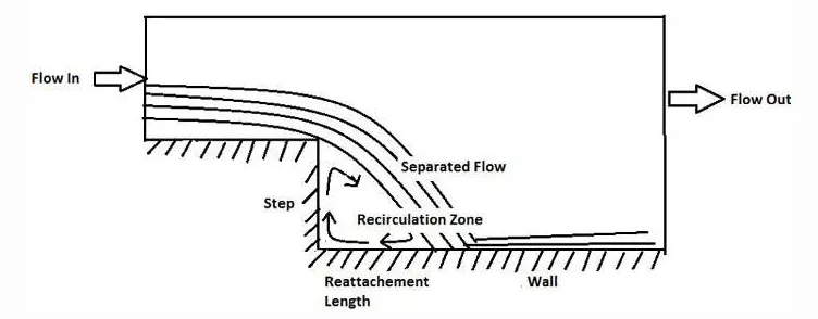
Fig1: Backward Facing Step geometry
Case Setup:
1. The following geometry was imported and the boundaries were flagged.
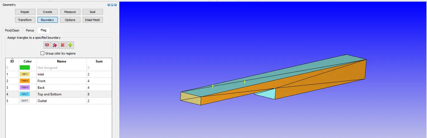
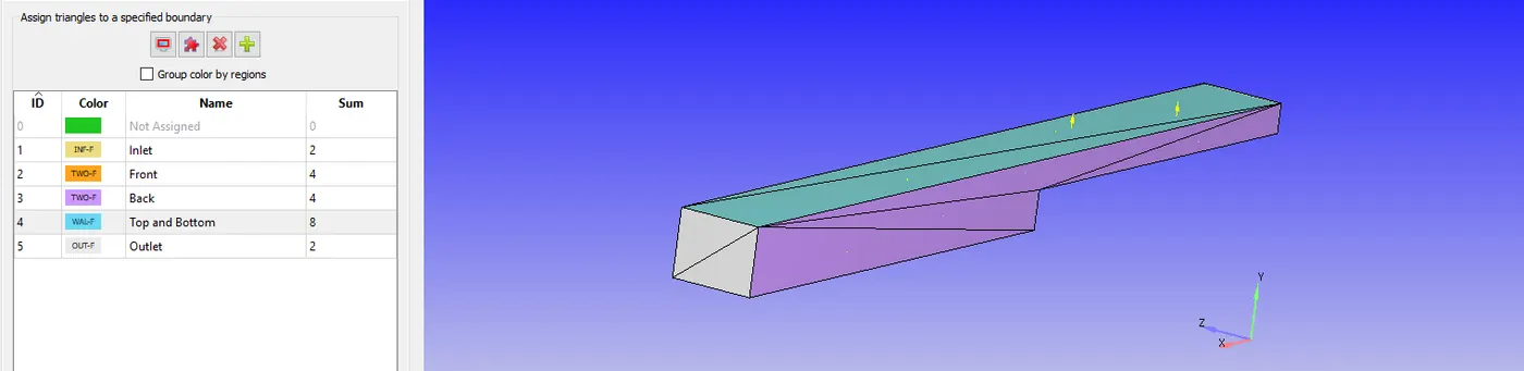
Run a diagnosis check to confirm the imported geometry doesn't have any errors.
Check the direction of normals, make sure all the normals are facing inwards, i.e. towards the fluid domain. (Note: in the above picture the arrow seen on the top face is actually the normal of the bottom face)
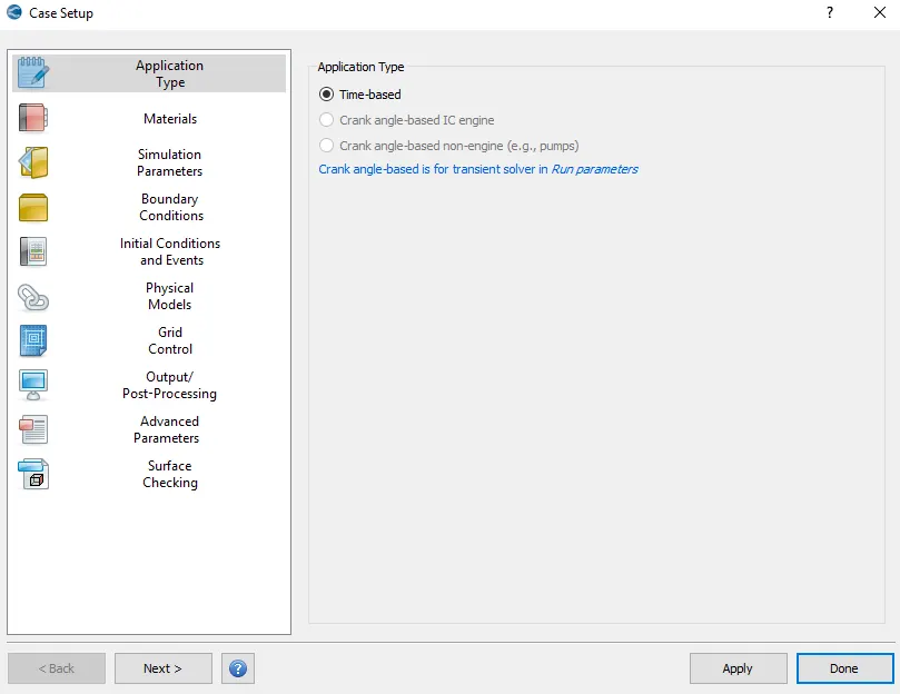
2. Application Type
3. Materials
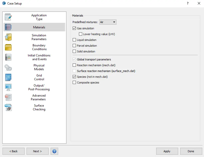
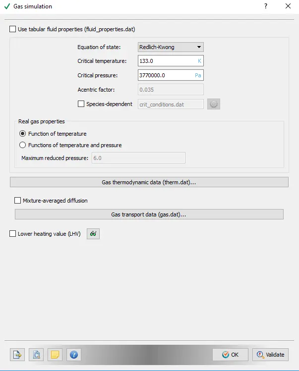
3.1. Gas simulation
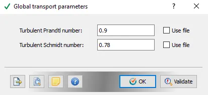
3.2. Global Transport parameters
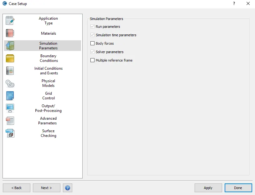
4. Simulation parameters
4.1. Run parameters
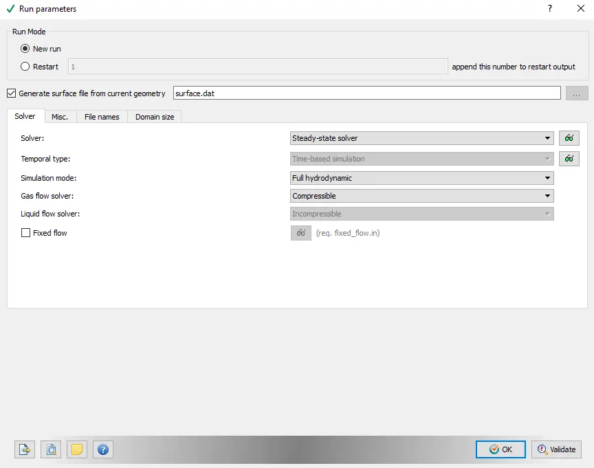
The simulation was solved using a steady-state solver.
4.1.1. Steady-state monitor
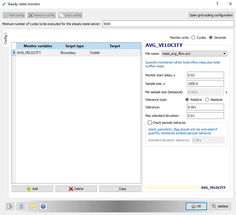
The minimum number of cycles to be completed is 5000. After which, convergence will be decided upon the tolerance value of 0.001,
4.2. Simulation time parameters
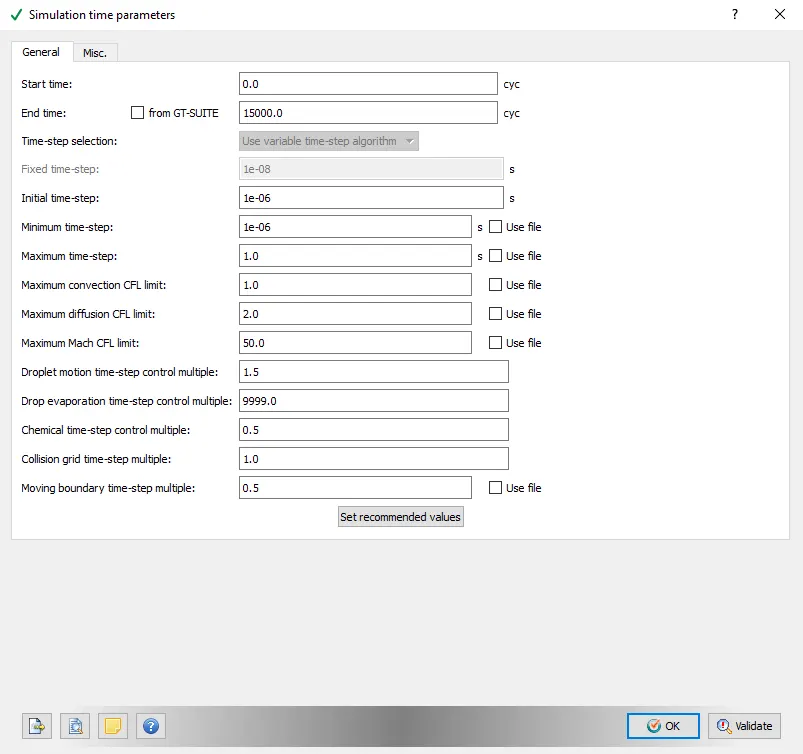
The simulation was conducted for 15,000 cycles with a minimum time-step of 1e-6 and a maximum time-step of 1. The maximum convection CFL limit is also 1.
4.3. Solver parameters
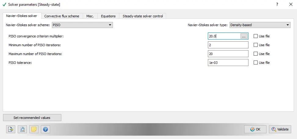
A PISO solver scheme was used. A density-based solver type was used.
5. Boundary Conditions
5.1. Inlet
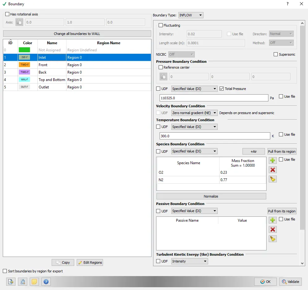
Inlet pressure of 110325 Pa was provided.
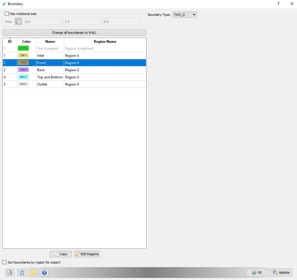
5.2. Front and Back
5.3. Top and Bottom
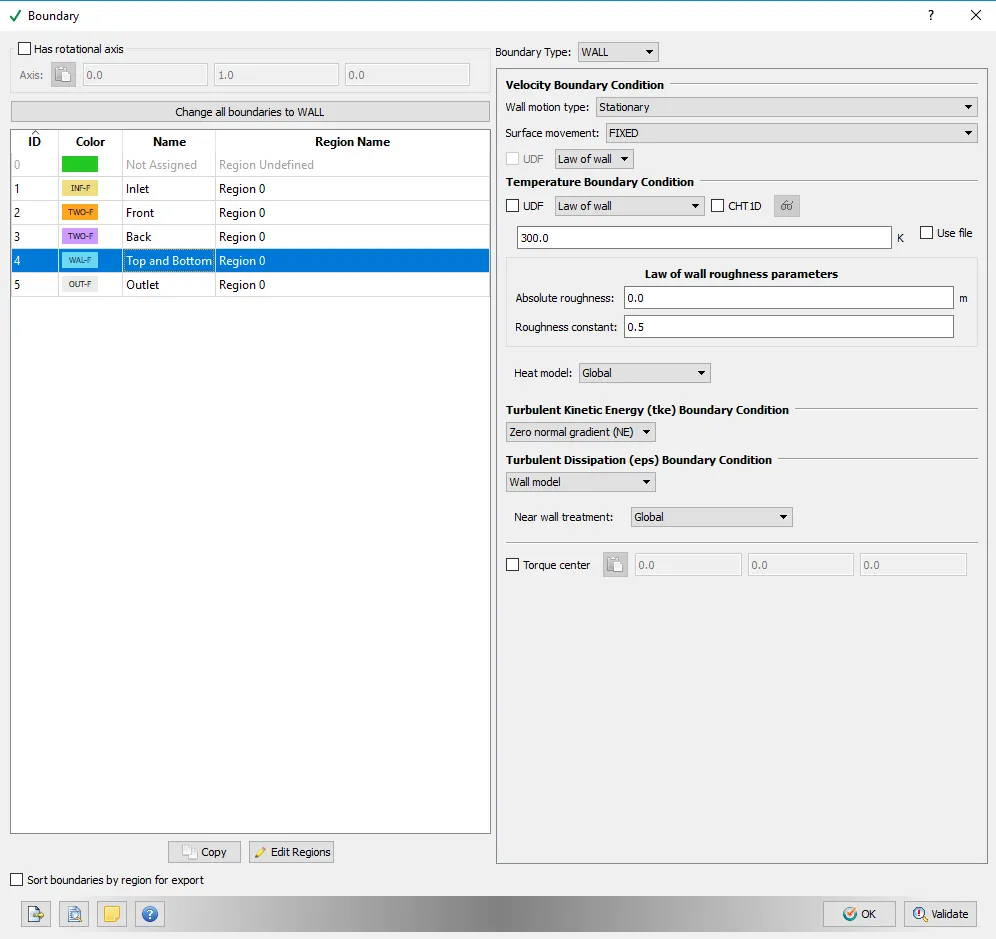
Top and Bottom walls obey the law of wall temperature and velocity boundary conditions.
5.4. Outlet
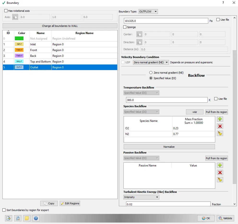
Outlet pressure is ambient condition.
6. Regions and Initialization
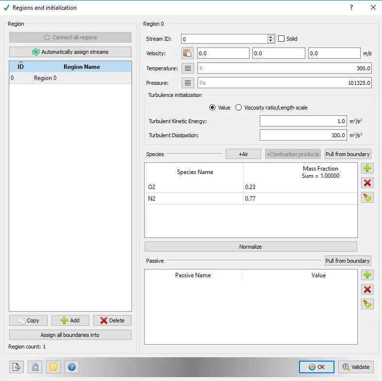
A region was created which consists of air(N2, O2) as material.
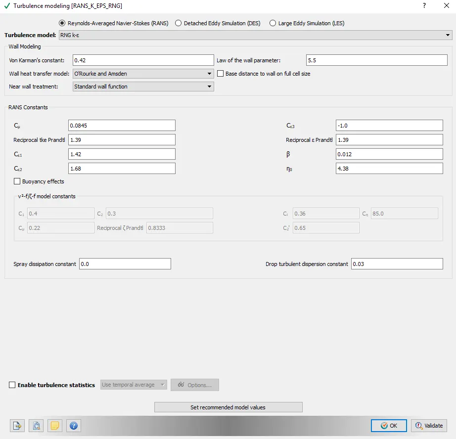
7. Turbulence modeling
8.1. Base Grid
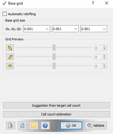
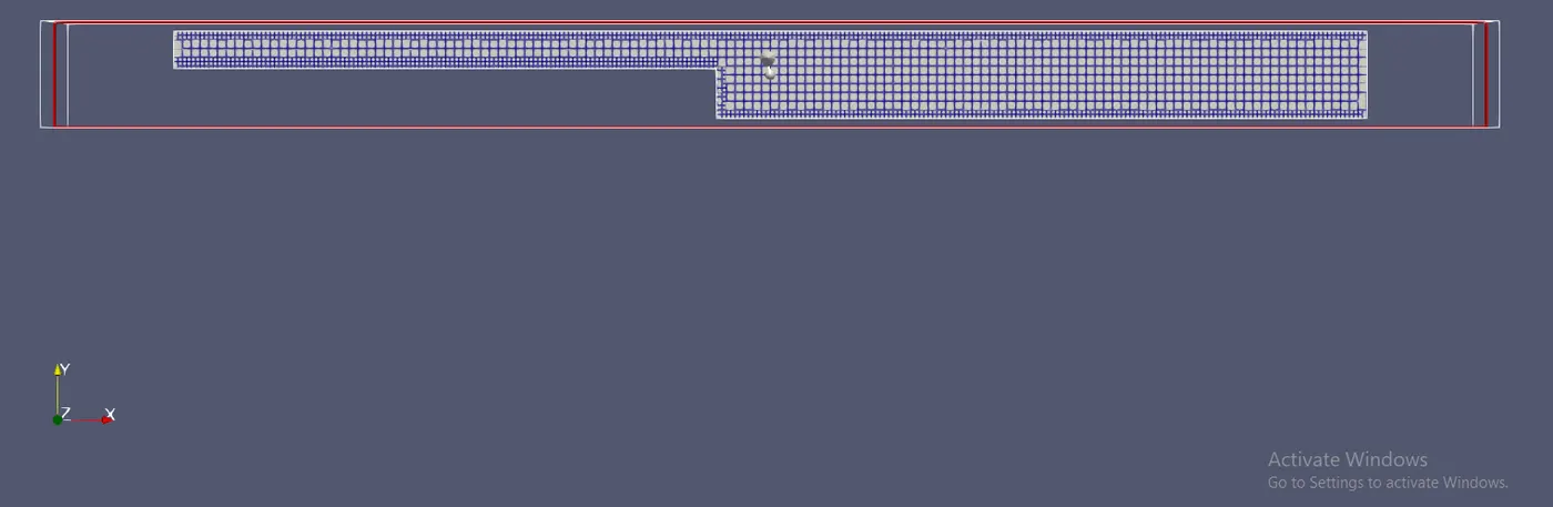
The simulation was conducted for 3 different mesh sizes 2e-3, 1.5e-3, 1e-3.
8.2. Fixed Embedding
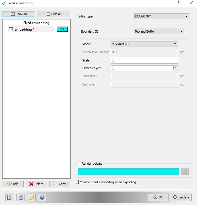
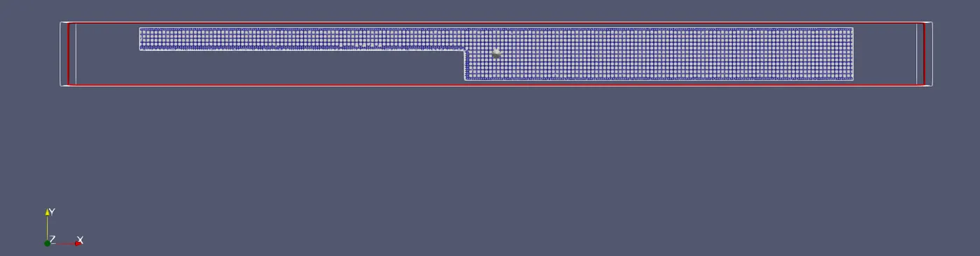
Embedding is provided for finer refined mesh at the boundaries.
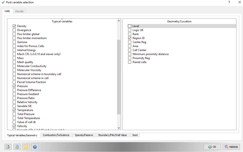
9.1. Post variable selection
9.2. Output files
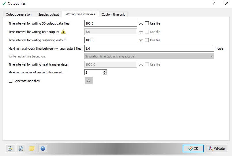
Since we are conducting simulation for 15,000 cycles it can save output files for a maximum of 150 times before the tolerance values are met(i.e. solution converged).
The Input files were exported to a folder and solved using Cygwin terminal commands.
The output files which were obtained after solving were post-processed into EnSight file type, which can be then opened in Paraview.
Results:
1. Mesh 1: 2e-3 m
1.1. Mesh picture
1.2. Cell count
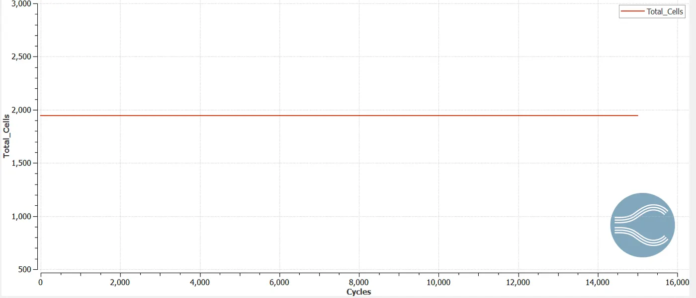
The cell count for mesh 1 is 1943.
1.3. Pressure contour
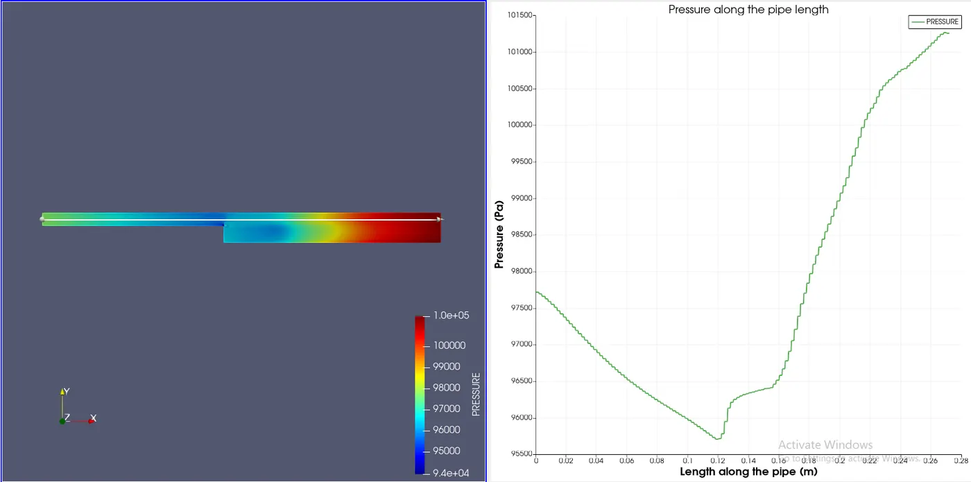
The pressure initially decreases in the constant cross-section area. But, when the step is encountered, the pressure again starts to increase and keeps increasing till the end.
1.4. Velocity contour
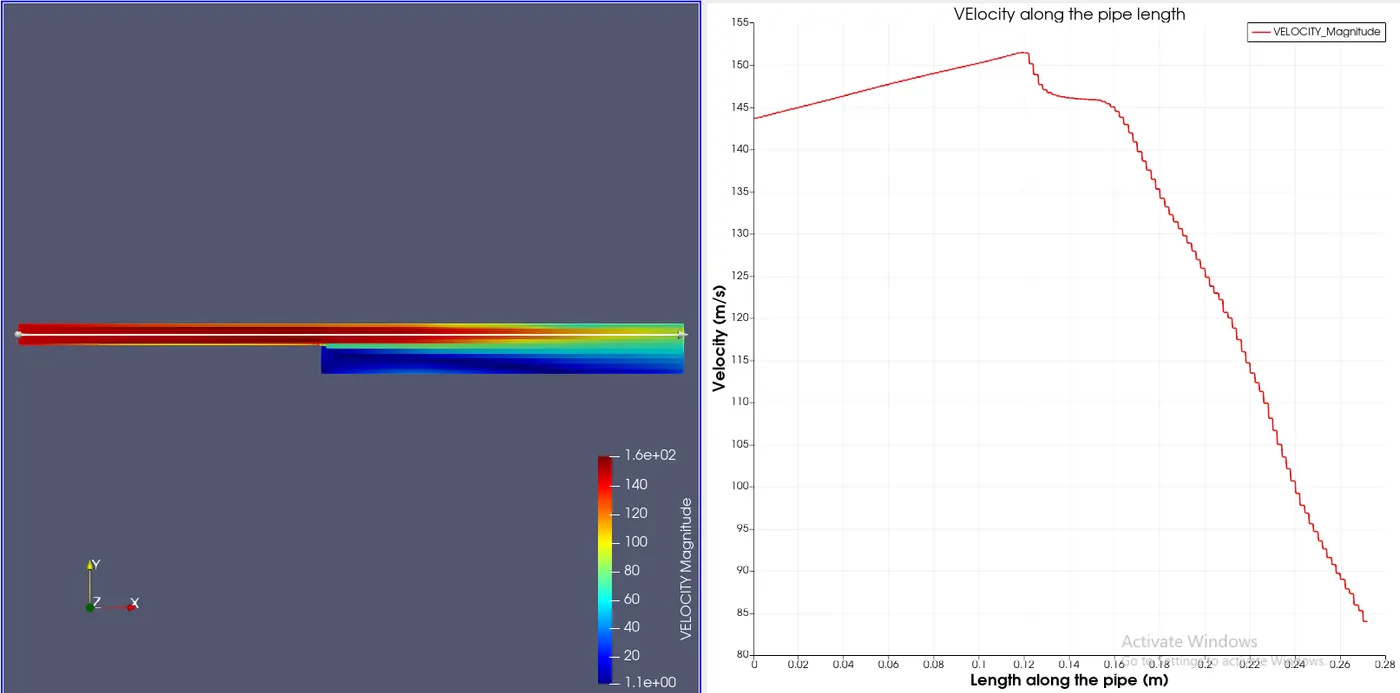
The velocity initially increases in the constant cross-section area. But, when the step is encountered the velocity starts to decrease rapidly till the end.
1.5. Pressure plot
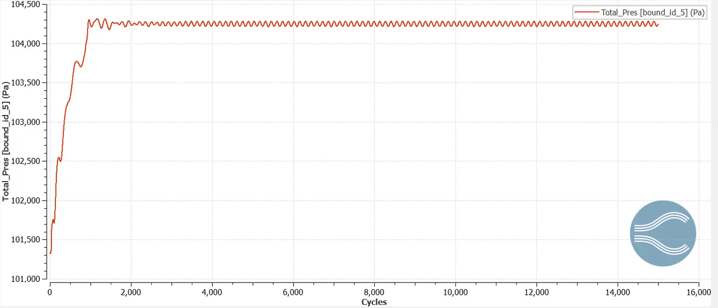
The total pressure at the outlet is 104,236 Pa.
1.6. Velocity plot
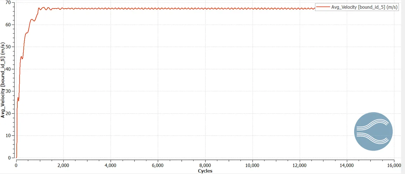
The average velocity at the outlet is 66.9319 m/s.
1.7. Mass flow rate plot
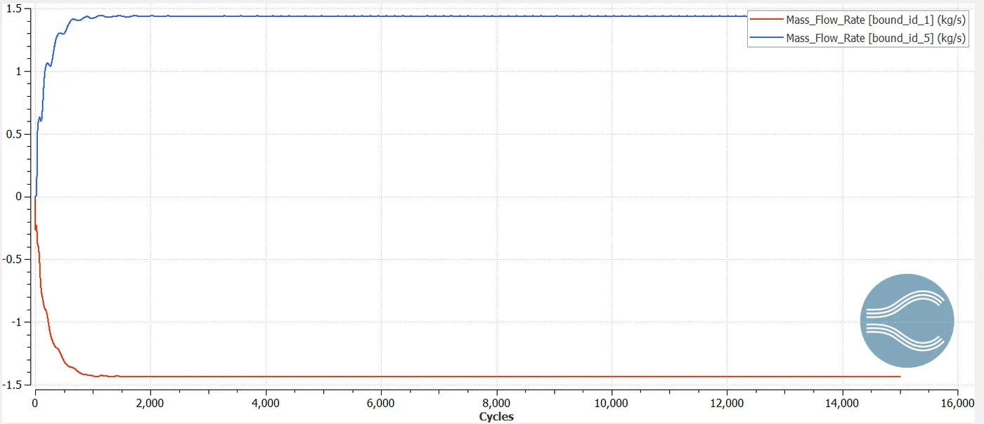
The mass flow rate at the inlet is -1.43505 kg/s and the mass flow rate at the outlet is 1.43716 kg/s.
2. Mesh 1: 2e-3 m
2.1. Mesh picture
2.2. Cell count
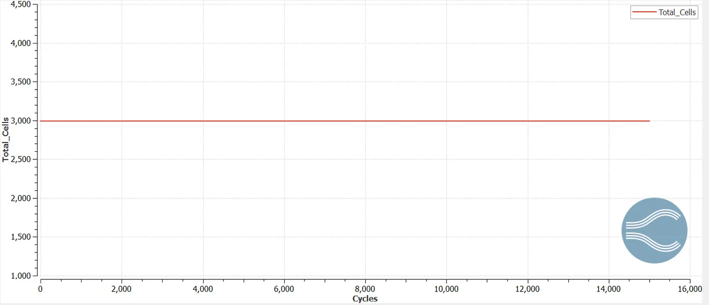
The cell count for mesh 2 is 2994.
2.3. Pressure contour
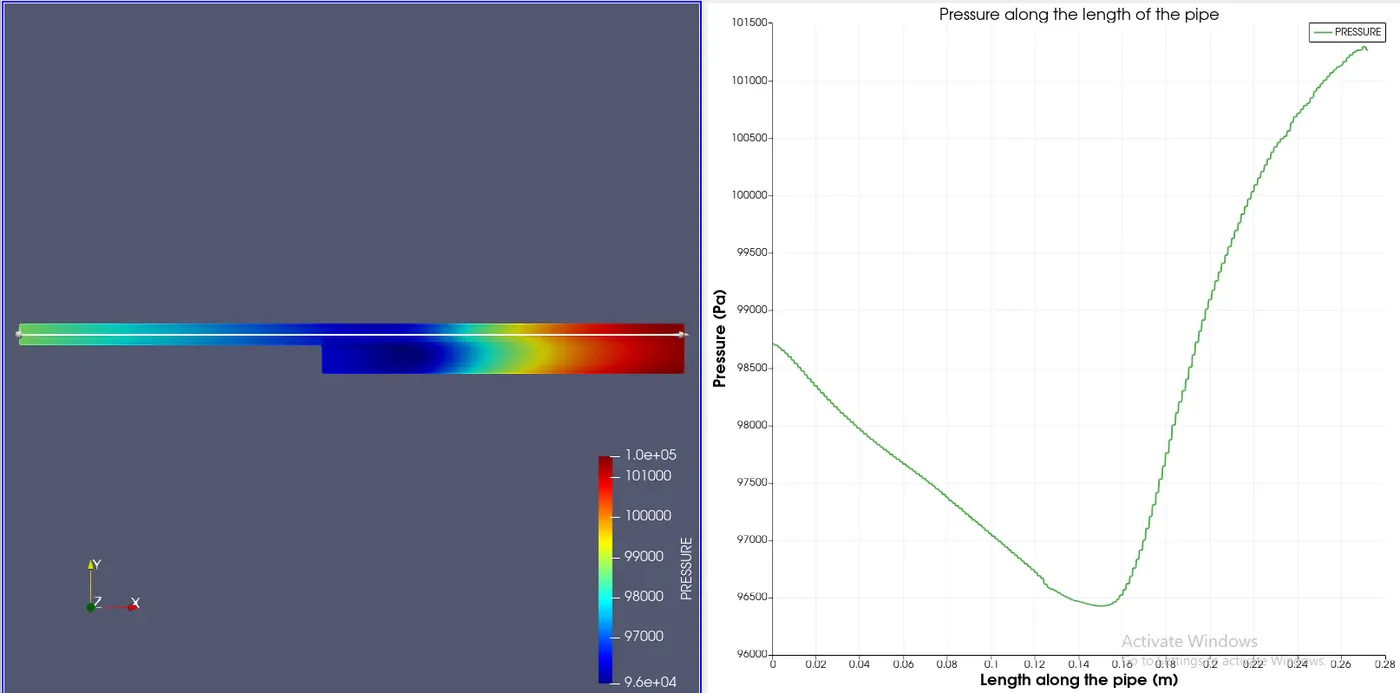
The pressure initially decreases in the constant cross-section area. But, when the step is encountered, the pressure again starts to increase and keeps increasing till the end.
2.4. Velocity contour
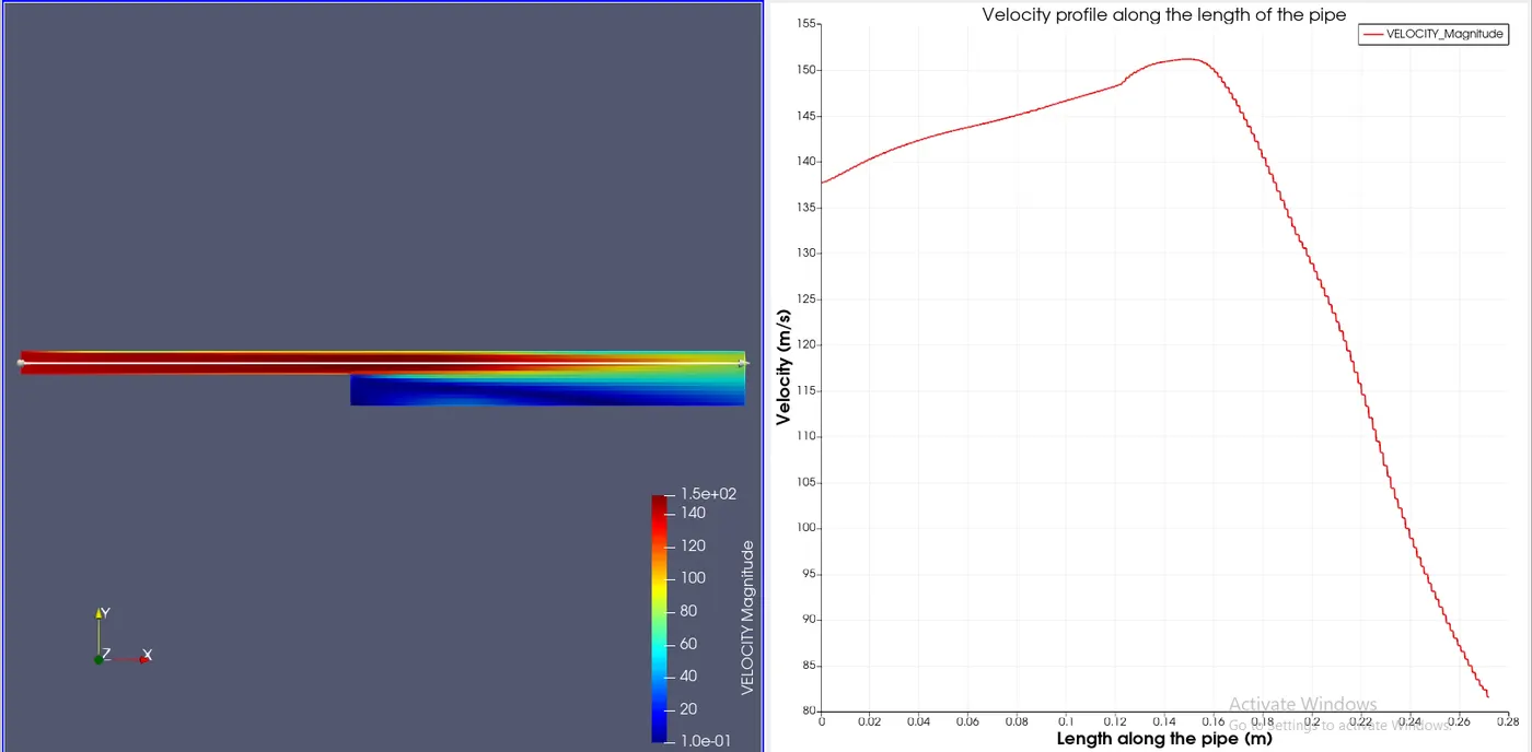
The velocity initially increases in the constant cross-section area. But, when the step is encountered the velocity starts to decrease rapidly till the end.
2.5. Pressure plot
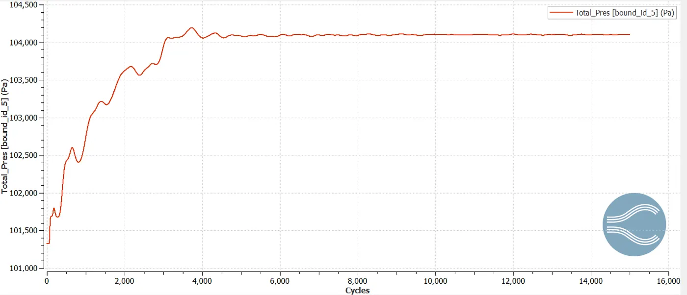
The total pressure at the outlet is 104,104 Pa.
2.6. Velocity plot
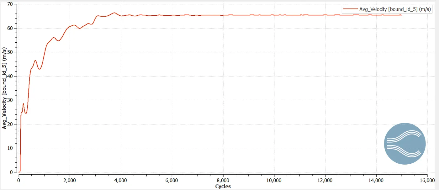
The average velocity at the outlet is 65.4141 m/s.
2.7. Mass flow rate plot
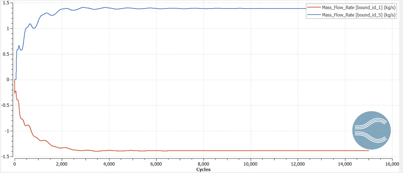
The mass flow rate at the inlet is -1.38725 kg/s and the mass flow rate at the outlet is 1.38715 kg/s.
3. Mesh 1: 2e-3 m
3.1. Mesh picture
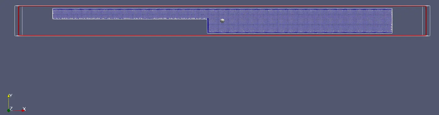
3.2. Cell count
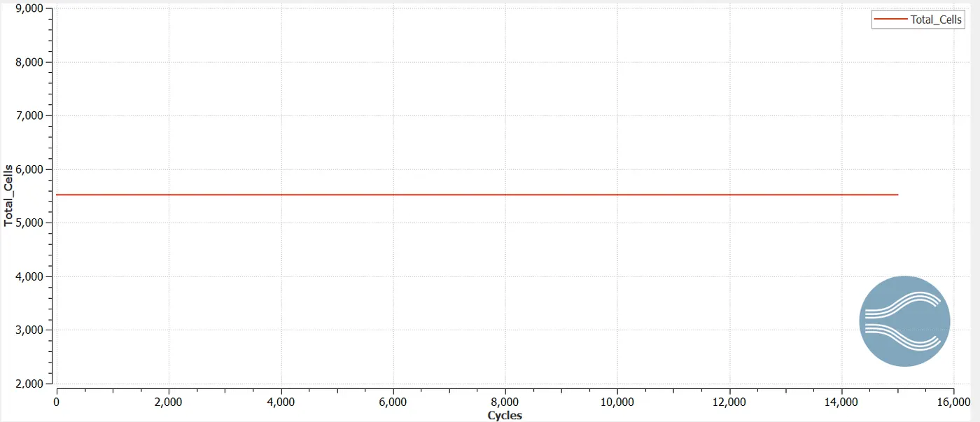
The cell count for mesh 3 is 5516.
3.3. Pressure contour
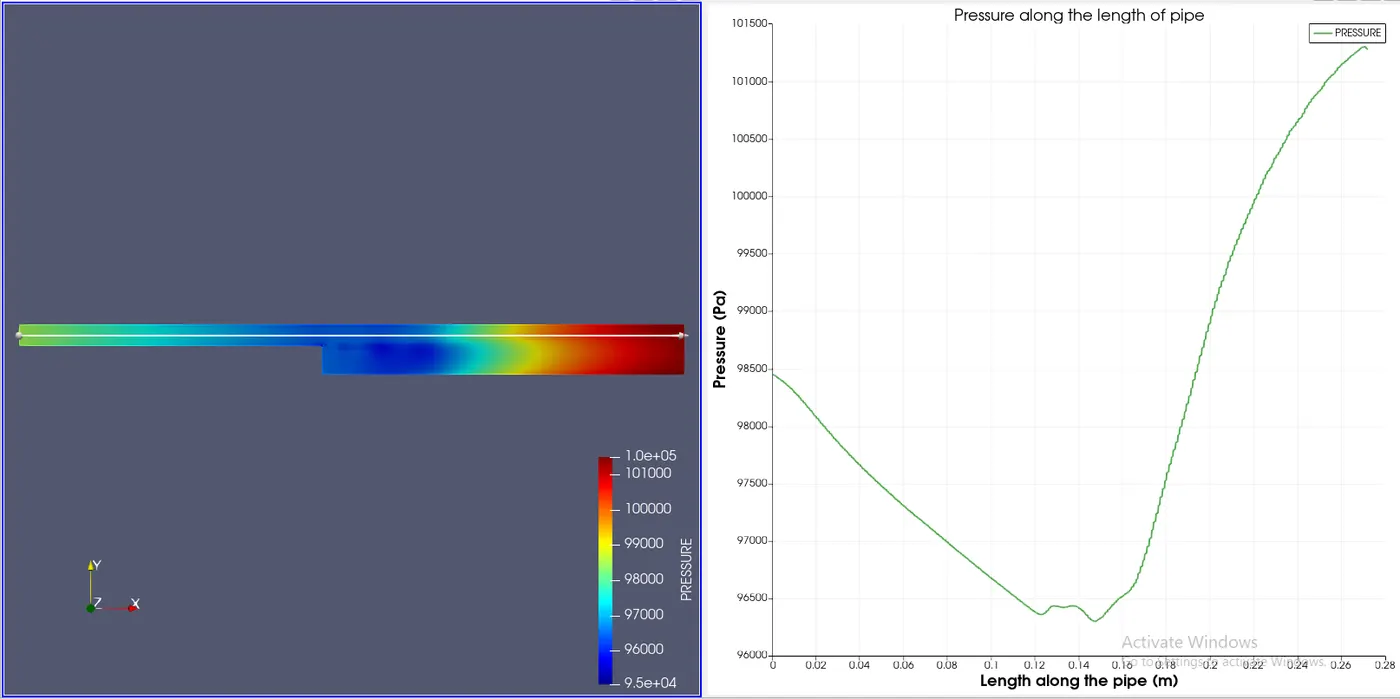
The pressure initially decreases in the constant cross-section area. But, when the step is encountered, the pressure again starts to increase and keeps increasing till the end.
3.4. Velocity contour
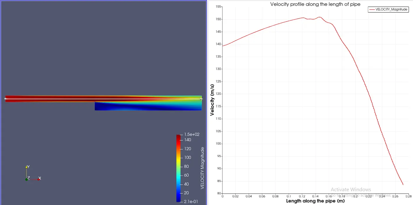
The velocity initially increases in the constant cross-section area. But, when the step is encountered the velocity starts to decrease rapidly till the end.
3.5. Pressure plot
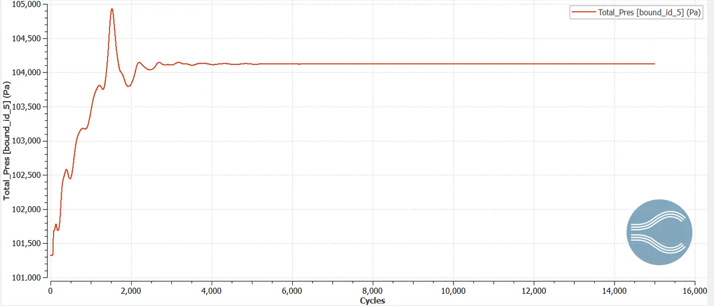
The total pressure at the outlet is 104,123 Pa.
3.6. Velocity plot
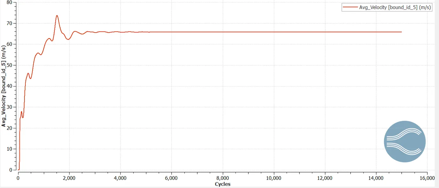
The average velocity at the outlet is 65.7807 m/s.
3.7. Mass flow rate plot
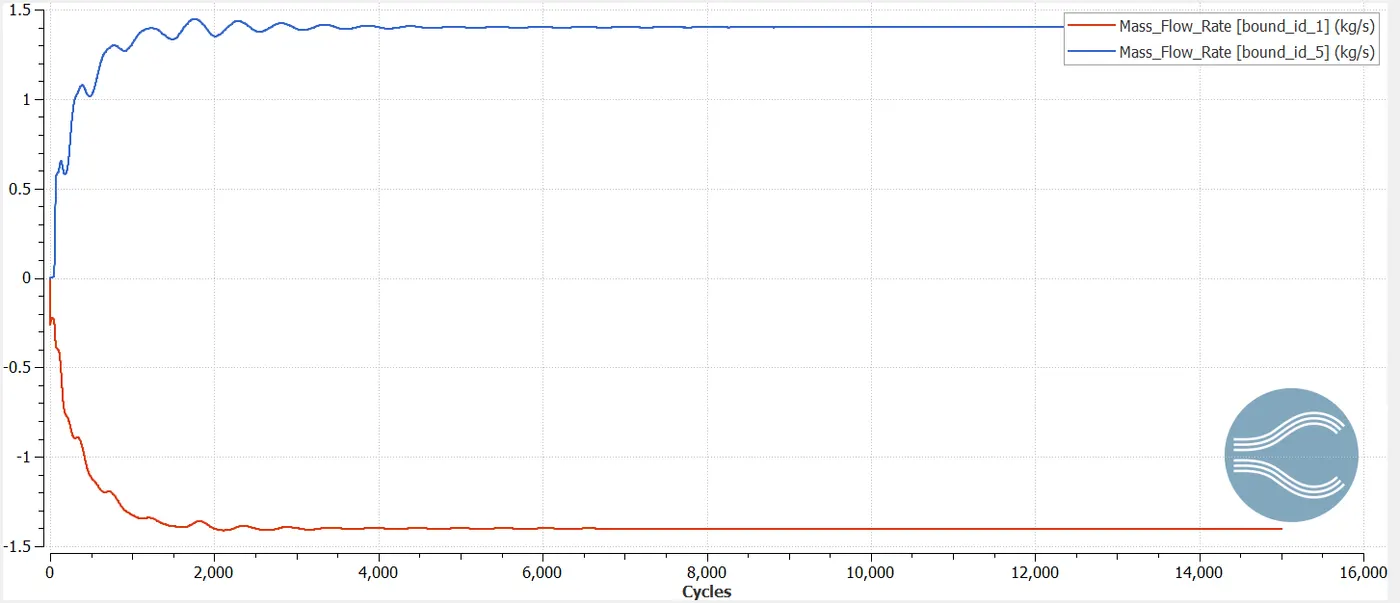
The mass flow rate at the inlet is -1.40058 kg/s and the mass flow rate at the outlet is 1.40072 kg/s.
Animation:
1. Velocity animation:
From the velocity animation, we can see that the domain was blue entirely(i.e. zero velocity), then as the iterations are solved the velocity develops throughout the domain, and we get a steady-state solution of velocity contour, wherein the velocity initially increases, but after the step, there is a decrease in velocity.
2. Pressure animation:
From the pressure animation, we can observe the domain was red entirely(i.e. the inlet pressure), but as the iterations are being solved the pressure develops throughout the domain, and we get a steady-state solution of pressure contour, wherein the pressure initially decreases in the constant cross-section area, but after the step was encountered, the cross-section area increases abruptly which causes an increase in pressure.
Flow Separation:
Flow separation is the point at which the velocity gradient at the surface in a direction normal to the wall decreases to zero. It may happen due to viscosity, pressure gradient, or abrupt change in geometry. In BFS, it happens due to an abrupt change in geometry. Flow separation creates a recirculation zone wherein pressure is reduced and flow may reverse direction. After the recirculation zone, there is re-attachment.
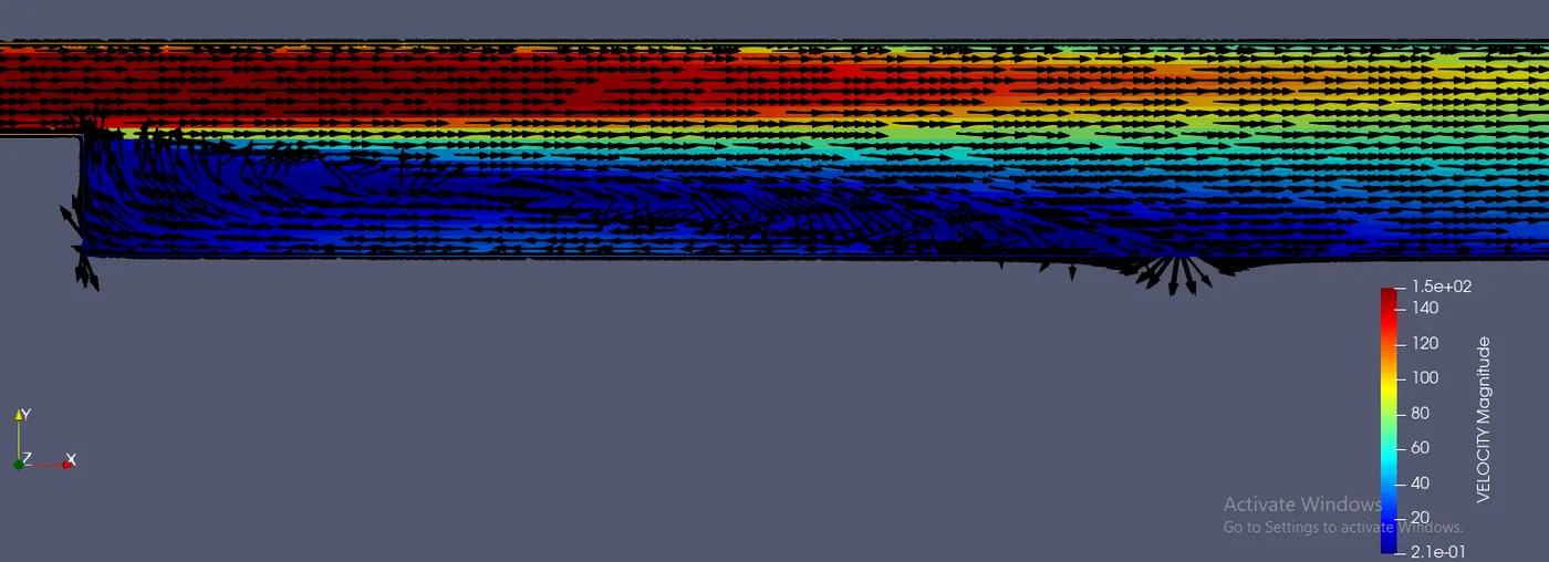
From the above figure, we can observe how the velocity vectors change direction and finally get reversed in the recirculation zone due to the pressure gradient.
Where flow separation?
The flow separation occurs at the step, due to an abrupt change in geometry and adverse pressure gradient.
Why flow separation?
Flow separation is occurring also due to the abrupt change in geometry, because of which a low-pressure zone is created, which causes recirculation.
Conclusion:
1. The mass flow rate graph confirms the conservation of mass principle.
2. The average velocity and total pressure at the outlet is almost the same, for all the 3 meshes.
3. The flow separation was observed in the geometry.