Week 5: Prandtl Meyer Shock problem
Aim: To simulate the Prandtl-Meyer Shock flow in Converge CFD.
Theory:
1. What is a Shock wave?
A shock wave is a type of propagating disturbance that moves faster than the local speed of sound in the medium. Like an ordinary wave, a shock wave carries energy and can propagate through a medium but is characterized by an abrupt, nearly discontinuous, change in pressure, temperature, and density of the medium.
2. Shock flow boundary conditions
2.1. Dirichlet boundary condition
In the Dirichlet boundary condition, the value of the function is given at the boundary.
`y(x)=f(x)`
2.2. Neumann boundary condition
In the Neumann boundary condition, the value of a normal derivative of the function is specified.
`(del y)/ (del n) = f(x)`
2.3. Robin boundary condition
It is a weighted combination of the Dirichlet boundary condition and the Neumann boundary condition.
`c_1y + c_2 (del y)/(del n) = f`
Where `c_1` and `c_2` are constants.
2.4. Mixed boundary conditions
In mixed boundary conditions, the solution of the given equation is required to satisfy different boundary conditions on disjoint parts of the boundary of the domain where the condition is stated.
4. Why do we use Neumann BC at Outlet?
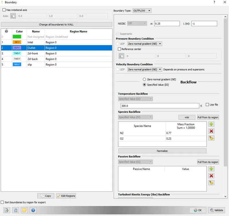
For a supersonic outlet, the characteristic curves propagate outside the domain, along with the streamline. Hence the values of the variable need to be floated, i.e. we calculate the values using linear extrapolation. Hence, we have used Zero normal gradient as the boundary condition for pressure and velocity.
5. Prandtl Meyer Shock
When an object moves faster than the speed of sound, and there is an abrupt decrease in the flow area, shock waves are generated. If the flow area increases, however, a different flow phenomenon is observed. If the increase is abrupt, we encounter a centered expansion fan. There are some marked differences between shock waves and expansion fans.
Across a shock wave, the Mach number decreases, the static pressure increases, and there is a loss of total pressure because the process is irreversible. As the flow across a shock is highly irreversible it cannot be approximated as isentropic. Through an expansion fan, the Mach number increases, the static pressure decreases, and the total pressure remain constant. Expansion fans are isentropic.
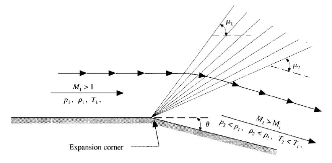
A Prandtl-Meyer expansion wave centered at the point of expansion corner is illustrated in the figure above. An expansion wave which is made up of several Mach waves fans out from the corner. The leading edge of the expansion fan makes an angle of `mu_1` with the upstream flow direction and the trailing edge of the wave makes an angle `mu_2`with respect to the downstream flow direction. These angles are called Mach angles and are defined as,
`mu_1 = sin^(-1)(1/M_1); mu_2 = sin^(-1)(1/M_2)`
Where `M_1 and M_2` are upstream and downstream Mach numbers respectively. As the flow passes through the expansion wave, the Mach number increases, and pressure, temperature, and density decrease. The flow upstream and downstream is always parallel to the wall.
Boundary Flagging:
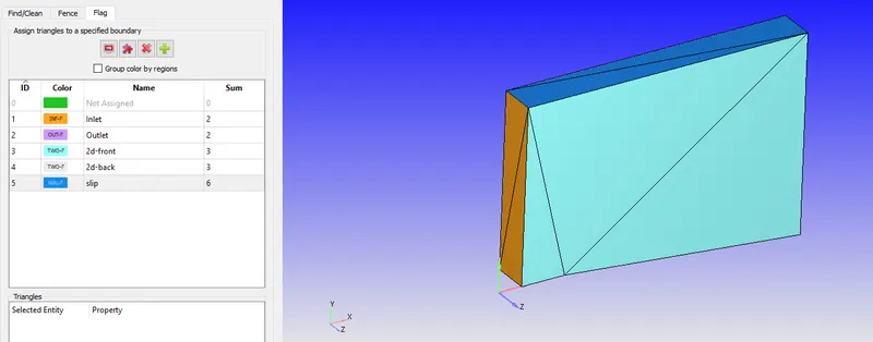
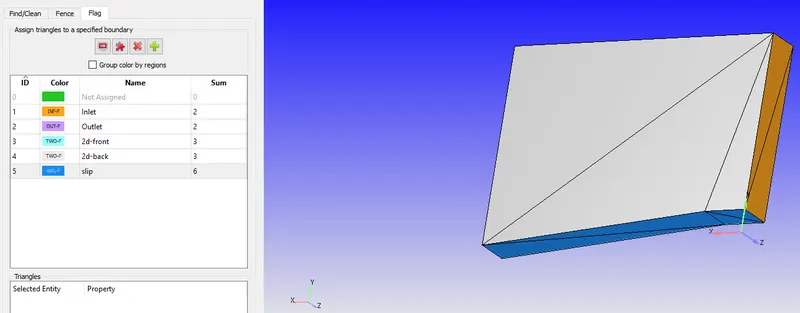
The geometry was scaled to mm, by dividing the entire geometry dimension by 1000.
Case Setup:
1. Application Type: Time-based.
2. Materials
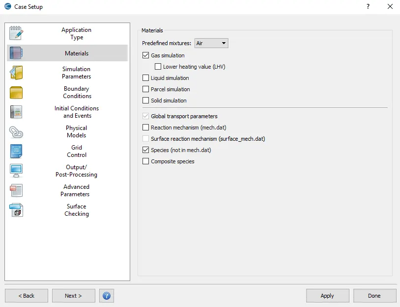
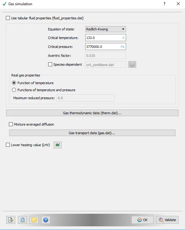
2.1. Gas simulation
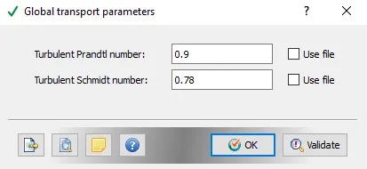
2.2. Global Transport parameters
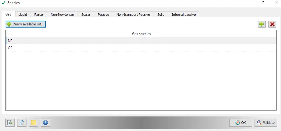
2.3. Species
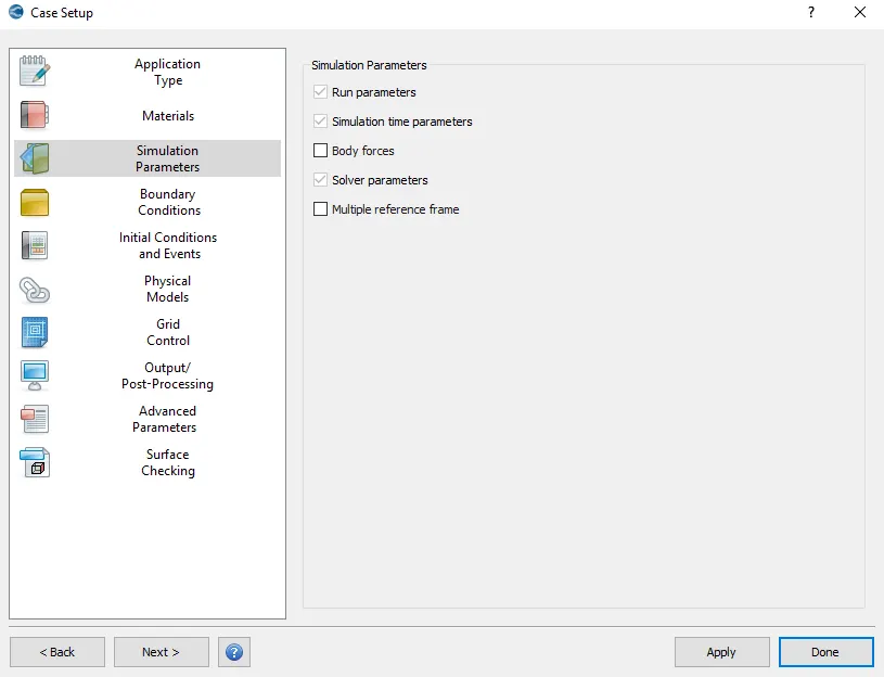
3. Simulation Parameters
3.1. Run parameters
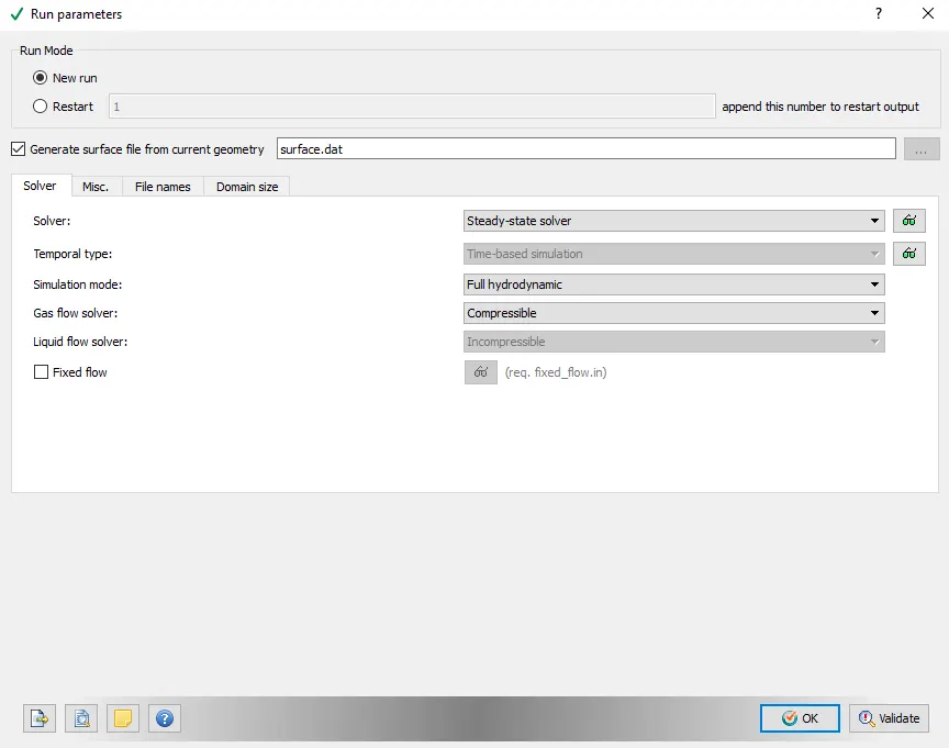
The shared memory was switched off.
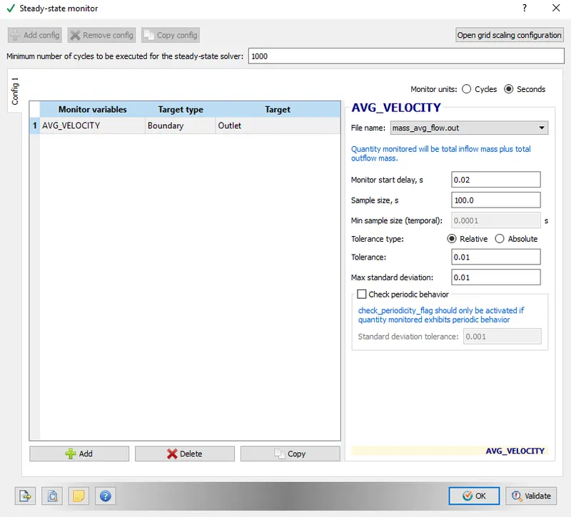
3.1.1. Steady-state monitor
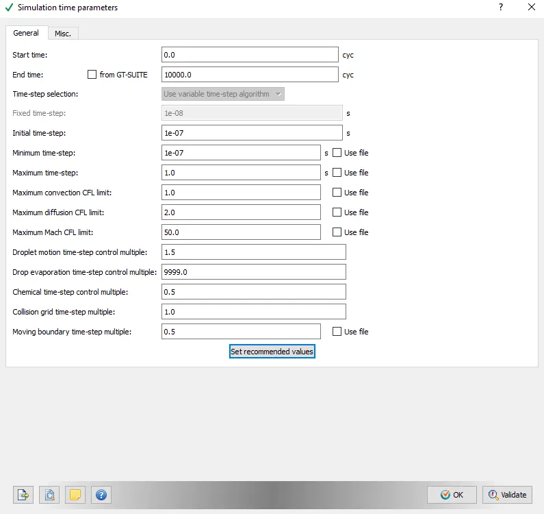
3.2. Simulation time parameters
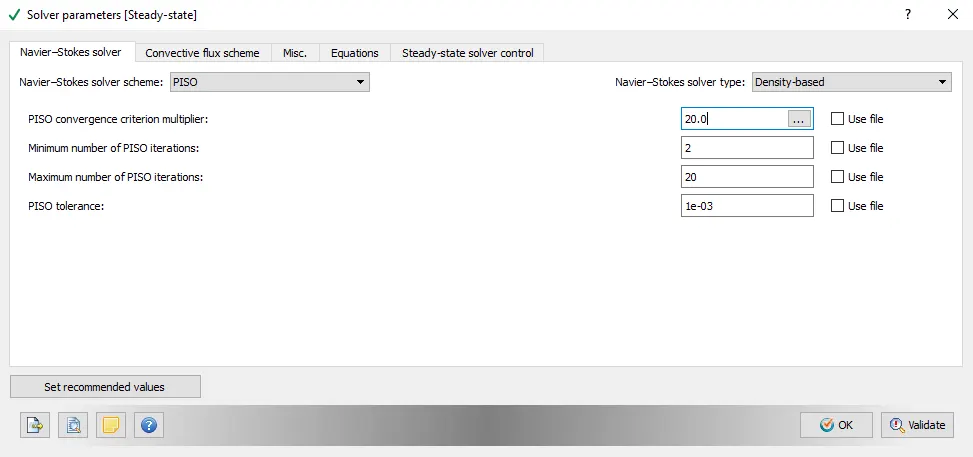
3.3. Solver parameters
4. Boundary Conditions
4.1. Inlet
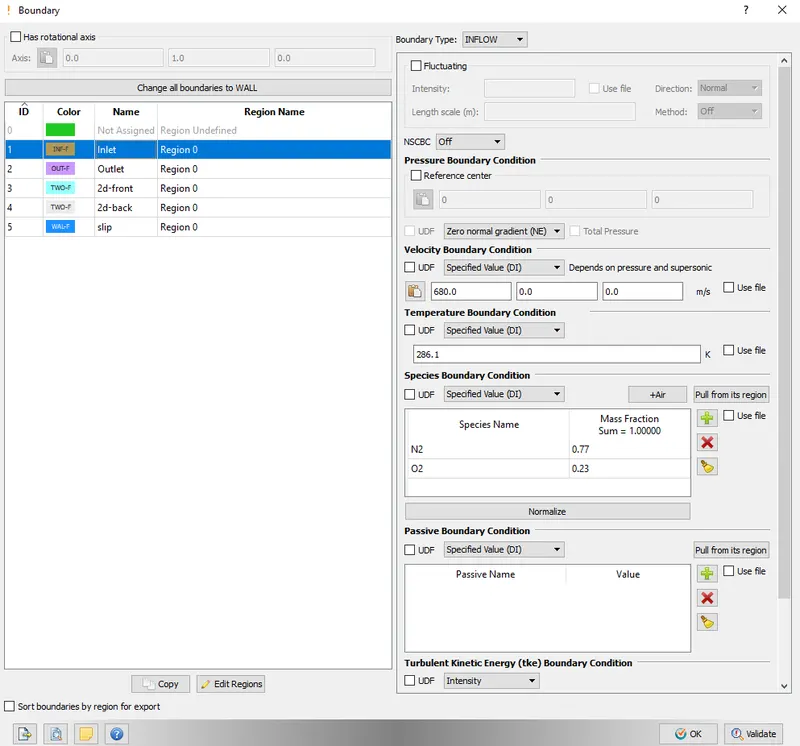
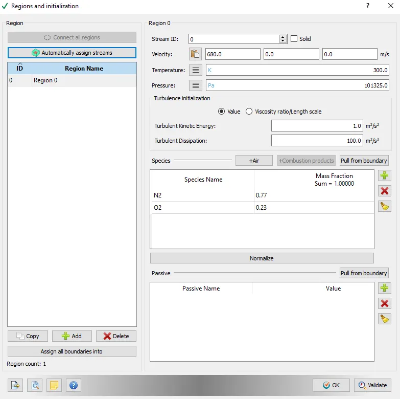
An inlet velocity of 680 m/s is provided at the inlet at a temperature of 286.1 m/s where the speed of sound is 340 m/s. Hence, the Mach Number at the inlet is approximately 2.
4.2. Outlet
4.3 2D Front and Back
4.4. Slip
5. Region Initialization
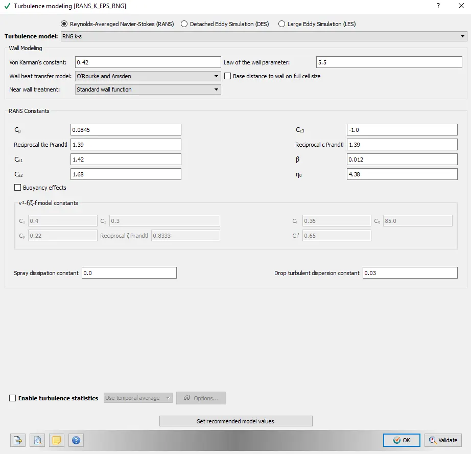
6. Turbulence modeling:
7. Grid Control
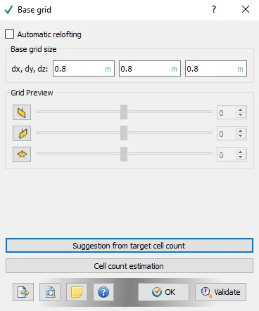
7.1. Base Grid
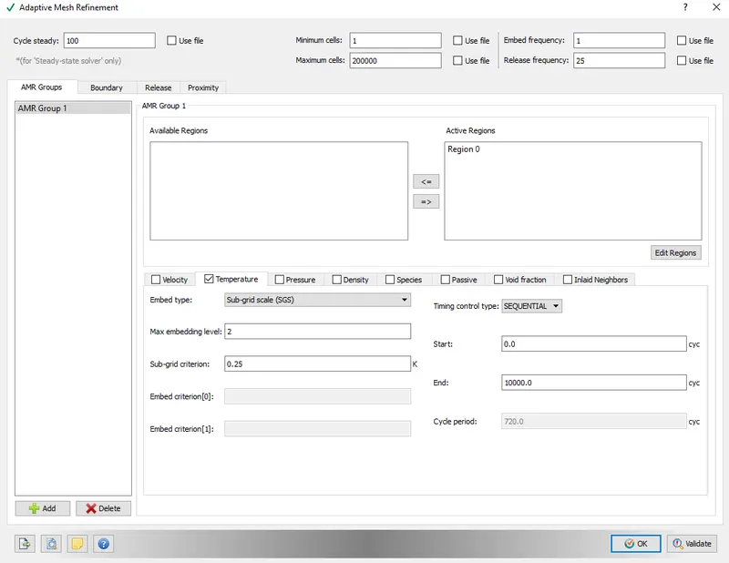
7.2. Adaptive Mesh Refinement
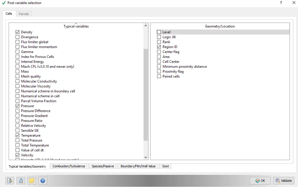
8. Output variables
9. Output files
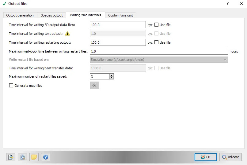
The input files were exported to a file and using Cygwin command line, we used converge-intelmpi solver to run a parallel simulation with 4 processors.
Using the post-processing tools, the output files obtained were converted into Ensight file type which can be then opened by ParaView.
Cases:
1. Velocity = 680 m/s and SGS Temperature sub-grid criteria = 0.1
2. Velocity = 680 m/s and SGS Temperature sub-grid criteria = 0.01
3. Velocity = 680 m/s and SGS Temperature sub-grid criteria = 0.001
4. Velocity = 100 m/s and SGS Temperature sub-grid criteria = 0.001
Results:
Case 1: Velocity = 680 m/s and SGS Temperature sub-grid criteria = 0.1
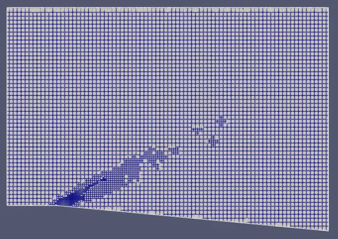
Mesh:
Cell Count:
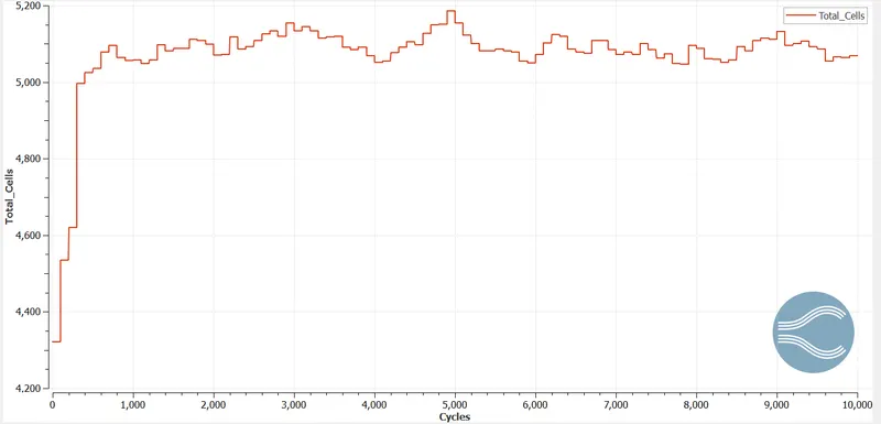
The cell count is 5120 cells.
Pressure Contour and plot:
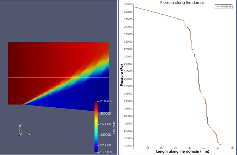
The pressure at the outlet is 210565 Pa.
Temperature Contour and plot:
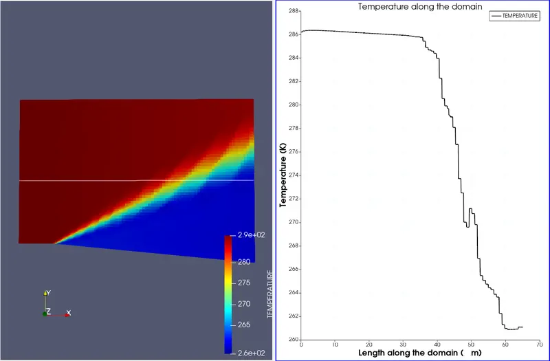
The temperature at the outlet is 261.091 K.
Velocity Contour and plot:
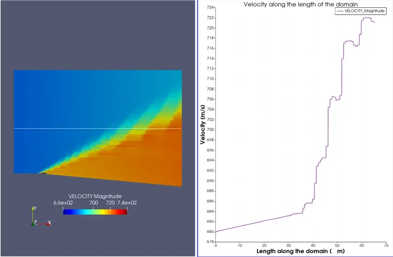
The velocity at the outlet is 720.974 m/s.
Density Contour and plot:
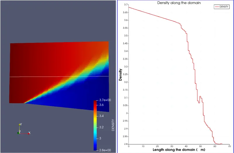
The density at the outlet is 2.80283 `(kg)/m^3`
Case 2: Velocity = 680 m/s and SGS Temperature sub-grid criteria = 0.01
Mesh:
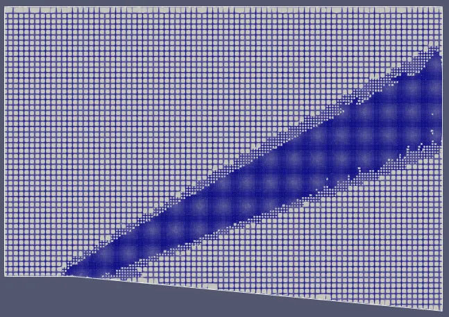
Cell Count:
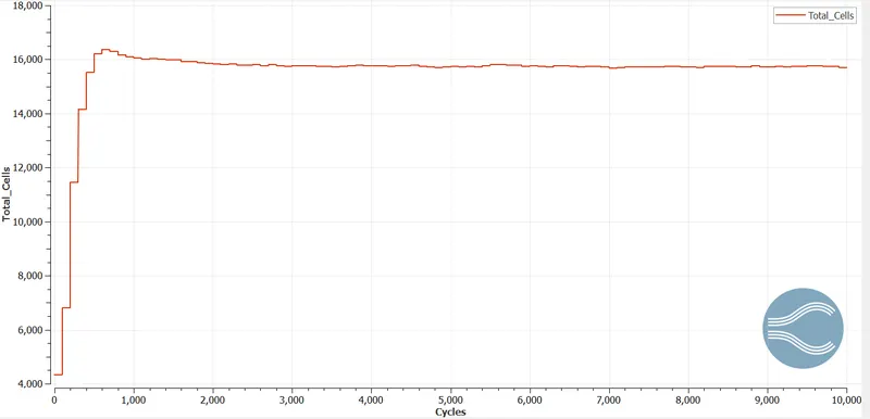
The cell count is 15,698 cells.
Pressure Contour and plot:
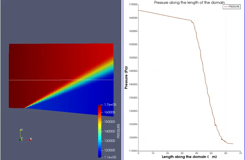
The pressure at the outlet is 117,708 Pa.
Temperature Contour and plot:
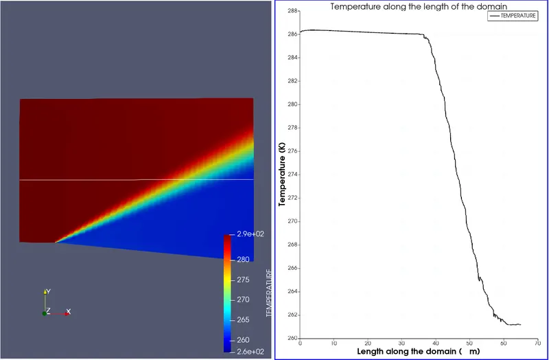
The temperature at the outlet is 261.226 K.
Velocity Contour and plot:
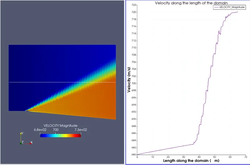
The velocity at the outlet is 720.085 m/s.
Density Contour and plot:
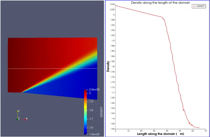
The density at the outlet is 1.56485 `(kg)/m^3`
Case 3: Velocity = 680 m/s and SGS Temperature sub-grid criteria = 0.001
Mesh:
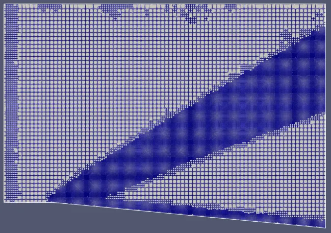
Cell Count:
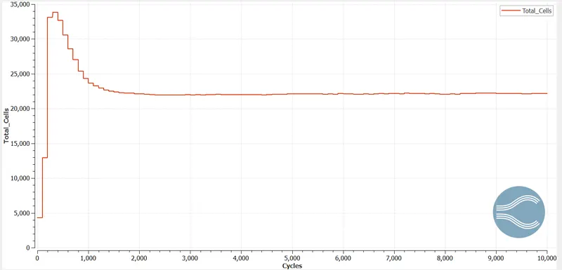
The cell count is 22,190 cells.
Pressure Contour and plot:
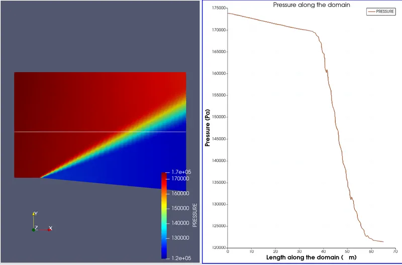
The pressure at the outlet is 121,434 Pa.
Temperature Contour and plot:
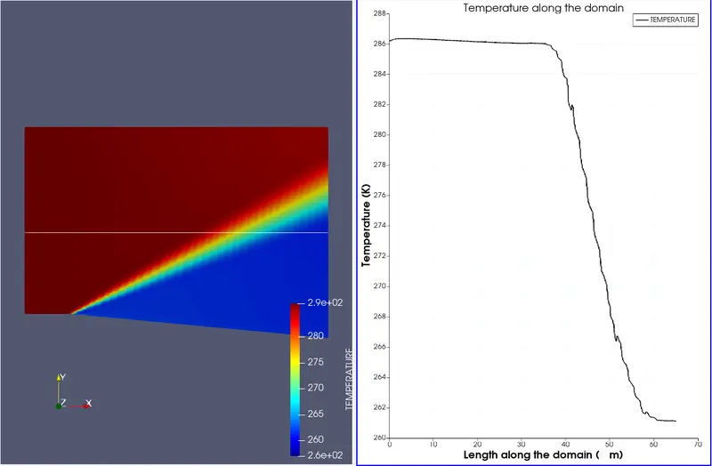
The temperature at the outlet is 261.135 K.
Velocity Contour and plot:
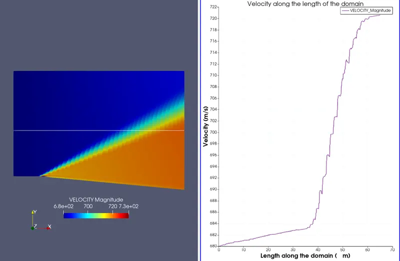
The velocity at the outlet is 720.574 m/s.
Density Contour and plot:
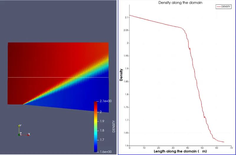
The density at the outlet is 1.61478 `(kg)/m^3`
Case 4: Velocity = 100 m/s and SGS Temperature sub-grid criteria = 0.01 and base mesh size = 0.4
Mesh:
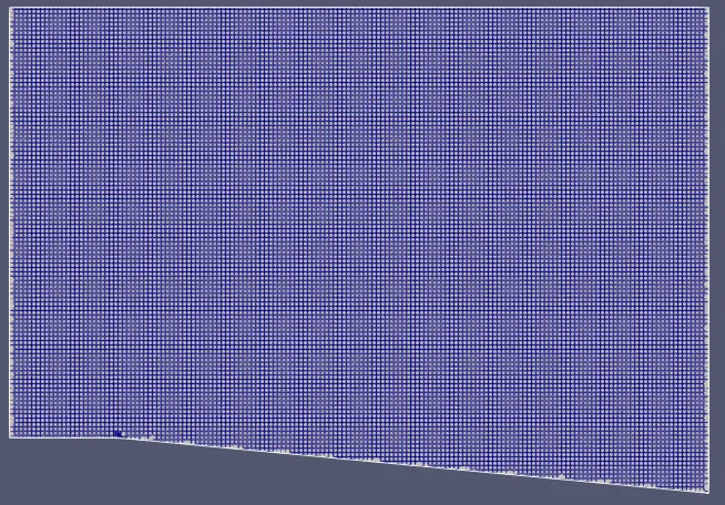
Cell count:
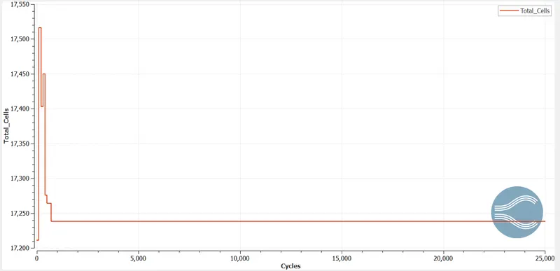
The cell count is 17,238 cells.
Pressure Contour and plot:
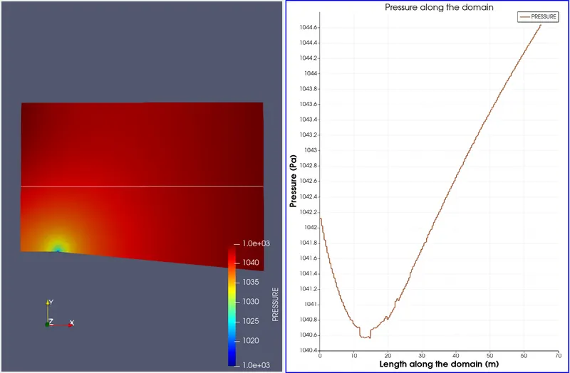
The pressure at the outlet is 2,085.03 Pa.
Temperature Contour and plot:
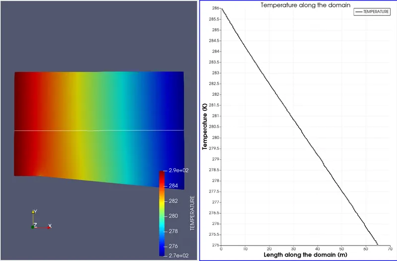
The temperature at the outlet is 275.052 K.
Velocity Contour and plot:
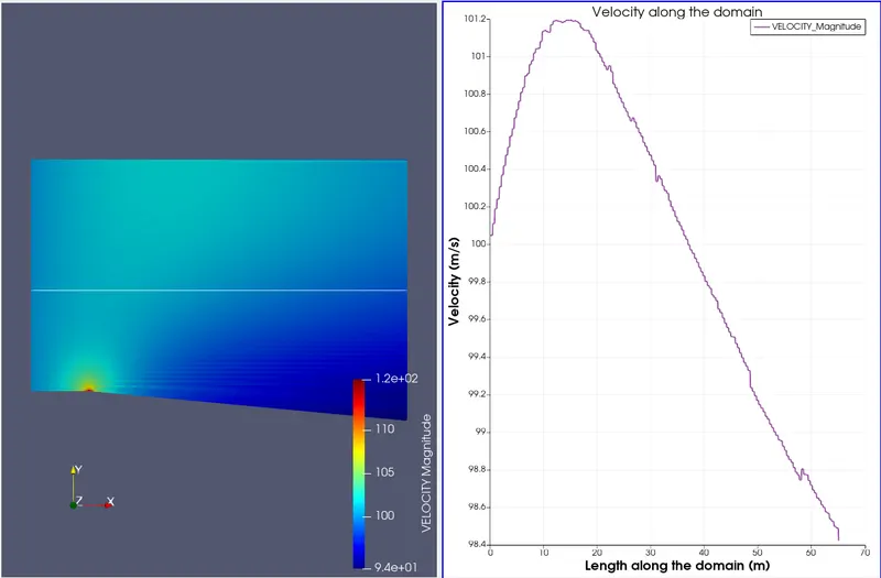
The velocity at the outlet is 98.423 m/s.
Density Contour and plot:
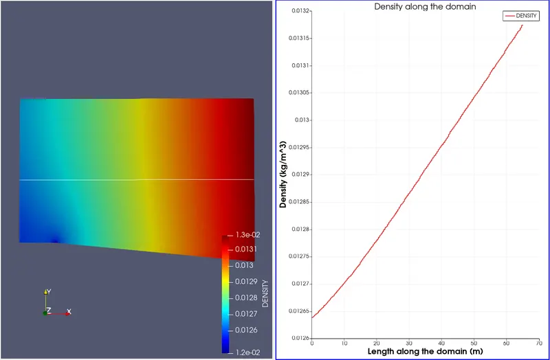
The density at the outlet is 0.0131739 `(kg)/m^3`
Animation:
1. Pressure
2. Temperature
3. Velocity
4. Density
Conclusion:
1. Temperature Sub-grid-scale of 0.01 is able to capture the Mach waves better than 0.1 and 0.001 which under-capture and over-captures respectively.
2. The cell-count increases when we decrease the temperature sub-grid scale criteria.
3. The pressure, temperature, density decrease across the Mach waves, however the velocity increases, for the supersonic inlet.
4. The 0.1 Temperature Sub-grid-scale criteria isn't able to capture the Mach wave properly hence the pressure value does not decrease as much as it should.
5. By increasing the cell-count i.e. by reducing the Temperature Sub-grid-scale criteria, we are able to capture the shock more accurately, because of the cell-count in and around the shock increases.
6. In the case of the Subsonic inlet, there is no formation of Mach waves around the expansion corner as expected. Since the cross-sectional area increases past the corner, the flow velocity close to the corner increases rapidly locally, thus proving the law of conservation of mass, since the mass flow rates will be equal at inlet and outlet. However, downstream the velocity decreases again, following Bernoulli's law. There is also a local reduction in pressure at the corner due to the local acceleration. At the outlet, finally, we get an increase in pressure, and velocity, temperature decrease along the domain.