Week 6 - Data analysis

DATA VISUALIZATION:

The given data file is VISUALIZED by using python program.

The program to read the file and to get the plots for the varies variables is

import math
import numpy as np
import matplotlib.pyplot as plt
from scipy.integrate import simps


column1=[]
column2=[]
column3=[]
column4=[]
column5=[]
column6=[]
column7=[]
column8=[]
column9=[]
column10=[]
column11=[]
column12=[]
column13=[]
column14=[]
column15=[]
column16=[]
column17=[]
label=[]
Units=[]

file = open('engine_data.out', 'r')
line_count = 1
for line in file:
        if '#' in line:
                if line_count is 3:
                         for j in range(1,18):
                                label.append(line.split()[j])
                if line_count is 4:
                         for k in range(1,18):
                                Units.append(line.split()[k])
                line_count = line_count + 1

        if '#' not in  line:
                columns=line.split()
                column1.append(float(columns[0]))
                column2.append(float(columns[1]))
                column3.append(float(columns[2]))
                column4.append(float(columns[3]))
                column5.append(float(columns[4]))
                column6.append(float(columns[5]))
                column7.append(float(columns[6]))
                column8.append(float(columns[7]))
                column9.append(float(columns[8]))
                column10.append(float(columns[9]))
                column11.append(float(columns[10]))
                column12.append(float(columns[11]))
                column13.append(float(columns[12]))
                column14.append(float(columns[13]))
                column15.append(float(columns[14]))
                column16.append(float(columns[15]))
                column17.append(float(columns[16]))

crank=column1
pressure=column2
max_pressure=column3
min_pressure=column4
mean_pressure=column5
max_temperature=column6
min_temperature=column7
volume=column8
mass=column9
density=column10
integrated_hr=column11
hr_rate=column12
c_p=column13
c_v=column14
gamma=column15
kinematic_viscosity=column16
dynamic_viscosity=column17




Inp = np.array([[0],crank, pressure,max_pressure,min_pressure,mean_pressure,max_temperature,min_temperature,volume,mass,density,integrated_hr,hr_rate,c_p,c_v,gamma,kinematic_viscosity,dynamic_viscosity])

print('\nEnter the engine parameters: ')
x = input("Engine parameter on the x axis: ")
x = int(x)
y = input("Engine parameter on the y axis: ")
y = int(y)
plt.plot(Inp[x],Inp[y])
plt.title(str(label[x-1]) + ' v ' + str(label[y-1]) + ' plot ')
plt.xlabel(str(label[x-1]) + str(Units[x-1]))
plt.ylabel(str(label[y-1]) + str(Units[y-1]))
plt.savefig(str(label[x-1]) + 'v' + str(label[y-1]))
plt.show()



#calculating area 
Area=simps(pressure,volume)
#area under the pv is equal to workdone by the engine
Workdone=(Area)
print(Workdone)
print(Area)
#power generated in an 4stroke engine
N=1500
z=2
p=(Workdone*2*np.pi*N)/(z*60*1000)
print(p)
#specific fuel consumption
#SFC=mass of fuel consumption/engine brake power
m=20*pow(10,-6)
SFC=(m*4)/(p*3600)
print(SFC)

        

RESULTS:

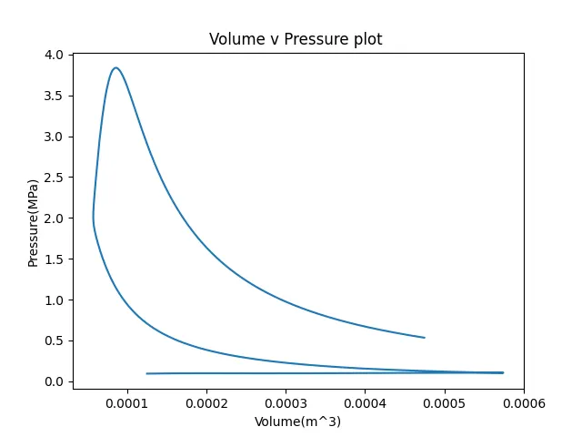
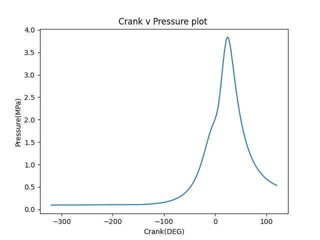
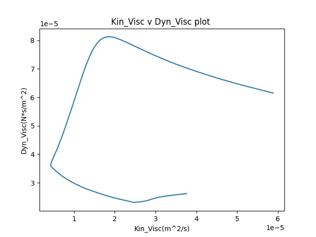
varies plots are:

P_V plot:

Crank vs pressure plot:

Kinematic viscocity vs Dynamic viscocity:

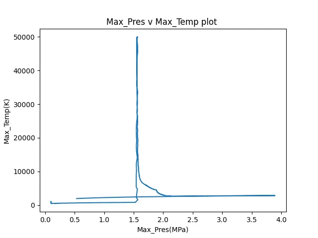
MAX_PRESSURE AND MAX TEMPERATURE:

Performance calculations:

1.Area under P_V plot is calculated by using simps imported from scipy.integration module the program for this is given above

The area under the curve gives the work done by the engine

2.The output power of the engine is given as `P=W*speed`

where W= workdone by the engine

W=Area under the p_v curve

N=speed is given as 1500RPM

`P=(W*N*2*PI)/(Z*60*1000)`

P in KW

Z=2 considering 4 stroke engine

3.Specific fuel consumption (SFV)(kg/kj)

SFV=mass of fuel consumption/engine power

mass of fuel consumption=20 micrograms per 1 stroke cycle.

SFV in kg/kJ

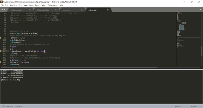
THE output is:

P_V Area=0.0005005

workdone=0.0005005

POWER in KW=3.93159*10e-5

SFV(KG/KJ)=0.00056522