Week 2 Air standard Cycle
Otto Cycle:
Otto Cycle is a constant volume cycle on which petrol and gas engines work.
The Otto cycle consists of 4 processes and are as follows.
- Process 1-2: Reversible Adiabatic Compression or Isentropic Compression
- Process 2-3: Constant Volume heat supply
- Process 3-4: Reversible Adiabatic Expansion or Isentropic Expansion
- Process 4-1: Constant Volume Heat Rejection
The explanation of above processes are as follows.
Process 1-2: Reversible Adiabatic Compression or Isentropic Compression:
The air is compressed into the clearance volume of the cylinder and thus raising the pressure and temperature of the air.
But, entropy remains constant as there is no heat transfer across the cylinder walls.
Process 2-3: Constant Volume heat supply (or) Heat Addition:
heat is supplied to air from hot body while the volume of the air remains constant.
Thus the work done is zero but the pressure and temperature of the air increase further to the maximum value attained in the cycle.
Due to heat supply(addition), there is an increase in entropy.
Qs = Cv(T3-T2)
Process 3-4: Reversible Adiabatic Expansion or Isentropic Expansion:
Air expands adiabatically causing the work-energy to be transferred to the surroundings at the expense of internal energy of the air.
Entropy remains constant as there is no heat transfer but the Pressure, Temperature and Volume decreases from stage 3 to 4.
Process 4-1: Constant Volume Heat Rejection
Heat is rejected from air to cold body. During the heat rejection, the air is maintained at constant volume and due to heat rejection, entropy decreases, pressure and temperature also decrease to initial state.
Thus, the cycle is completed.
Derivation of Otto Cycle:
derivation in order to calculate the efficiency of the Petrol engine by Otto Cycle.
Heat
Heat supplied during the process(2-3),Qs=Cv(T3-T2)
Heat rejected during the process(4-1),Qr=Cv(T4-T1)
Efficiency of otto cycle,`eta`=workdone/heat supplied
workdone=Qs-Qr
eta=Qs-Qr/Qs
=[Cv(T3-T2)-Cv(T4-T1)]/Cv(T3-T2)
=1-Cv(T4-T1)/Cv(T3-T2)
=1-(T4-T1)/(T3-T2)
Efficiency,eta=1-(T4-T1)/(T3-T2).
Compression ratio,r=volume before compression/volume after compression
Calculating the parameters from given values:
INPUTS:
pressure,p1=101325pa
Temperature at the input,T1=500k
Temperature after the compression,T3=2300k
cylinder bore =0.1mts
stroke length=0.1mts
connecting rod lenght=0.15
compression ratio,r=12
gamma=1.4
Volume computations:
stroke volume,Vs=pi/4*bore^2*stroke length
Compression volume,Vc=Vs/(r-1)
parameters at point 1
p1=101325pa
T1=500k
V1=Vs+Vc
parameters at point 2
V2=Vc
p1v1^gamma=p2v2^gamma(since adiabatic compression)
p2=p1*v1^gamma/V2^gamma
ideal gas equation
P1V1/T1=P2V2/T2
T2=P2*V2*T1/P1*V1
parameters at point 3
constant volume heat addition
V3=V2
T3=2300
ideal gas equation
P3V3/T3=P2V2/T2
P3=P2*V2*T3/T2*V3
parameters at point 4
V4=V1
P4V4^gamma=P3V3^gamma(since adiabatic expansion)
P4=P3*V3^gamma/V4^gamma
P4V4/T4=P3V3/T3(ideal gas equation)
T4=P4*V4*T3/P3*V3
hence we had computed all the values at four states of the cycle
efficiency =1-(T4_T1)/(T3-T2)
we draw a graph and analyse the parameters in the python program with different input values
To get the volume at each and value of the theta while compression and expansion is given as
V/Vc=1+0.5(r-1)*[R+1-cos(theta)-(R^2-sin(theta)^2)^0.5]
where R is constant =connecting rod length/a
a=crank pin radius
=stroke/2.
Thermal efficiency of engine:
let us assume
the specific heat at constant volume Cv=0.718J/kg
m=1kg
no of cylinders=1
z constant =2 for 4 stroke engine
workdone=heat supplied -heat removed
torque generated for one revolution
torque=workdone/2*pi*z
break power,pb(kw)=torque*omega
=torque*2*pi*N/60*1000
where N=revolutions per minute
Thermal efficiency=break power*mechanical efficiency/Fuel power.
The program is
import math
import matplotlib.pyplot as plt


def engine(bore,stroke,con_rod,cr,start_crank,end_crank):

	a=stroke/2
	R=con_rod/a
	v_s=math.pi*(1/4)*pow(bore,2)*stroke
	v_c=v_s/(cr-1)
	sc=math.radians(start_crank)
	ec=math.radians(end_crank)
	num_values=50
	dtheta=(ec-sc)/(num_values-1)
	V=[]
	for i in range(0,num_values):
		theta=sc+i*dtheta
		term1=0.5*(cr-1)
		term2=R+1-math.cos(theta)
		term3=pow(R,2)-pow(math.sin(theta),2)
		term3=pow(term3,0.5)
		V.append((1+term1*(term2-term3))*v_c)
	return V
#inputs
p1=101325
t1=500#crankpin radius

t3=2300
#geometric parameters
bore=0.1
stroke=0.1
con_rod=0.15
cr=12
gamma=1.4
#volume computation
v_s=((math.pi)/4)*pow(bore,2)*stroke
v_c=v_s/(cr-1)
v1=v_c+v_s

#state point2
v2=v_c
#p2v2^gamma=p1*v1^gamma
p2=(p1*pow(v1,gamma))/pow(v2,gamma)
#p2v2/t2=p1v1/t1
rhs=(p1*v1)/t1
t2=(p2*v2)/rhs
V_compression=engine(bore,stroke,con_rod,cr,180,0)
constant=p1*pow(v1,gamma)
#p_compression*V_compression^gamma=constant
p_compression=[]
for v in V_compression:
	p_compression.append((constant)/pow(v,gamma))

#state point 3
v3=v2
#p3v3/t3=p2v2/t2
rhs=(p2*v2)/t2
p3=(rhs*t3)/v3
V_expansion=engine(bore,stroke,con_rod,cr,0,180)
constant=p3*pow(v3,gamma)
#p_compression*V_compression^gamma=constant
p_expansion=[]
for v in V_expansion:
	p_expansion.append((constant)/pow(v,gamma))

#state point4
v4=v1
#p4v4^gamma=p3v3^gamma
p4=(p3*pow(v3,gamma))/pow(v4,gamma)
#p4v4/t4=p3v3/t3
rhs=p3*v3/t3
t4=p4*v4/rhs
# cycle efficiency
eta=1-((t4-t1)/(t3-t1))
# engine thermal efficiency
#assume
#constant volume specific heat
m=1
C_v=0.718
# four stroke engine z=2 constant,no of revolutions 2000
z=2
N=2000
#density of fuel petrol
density=0.71
#fuel consumed  in leaters per  hour
f=8
#workdone
workdone=m*C_v*(t3-t2-t4+t1)
#torque generated for one revolution
torque=(workdone)/(2*(math.pi)*z)
#breakpower inkw
breakpower=(torque*2*(math.pi)*N)/(60*1000)
#thermal efficiency of engine and engine having an mechanical efficiency of 0.8
ther_efficiency=(3600*breakpower*0.8)/(f*4800)
print(workdone)
print(torque)
print(breakpower)
print(ther_efficiency)
print(eta)
plt.plot([v2,v3],[p2,p3])
plt.plot(V_compression,p_compression)
plt.plot(V_expansion,p_expansion)
plt.plot([v4,v1],[p4,p1])
plt.xlabel('volume')
plt.ylabel('pressure')
plt.show()
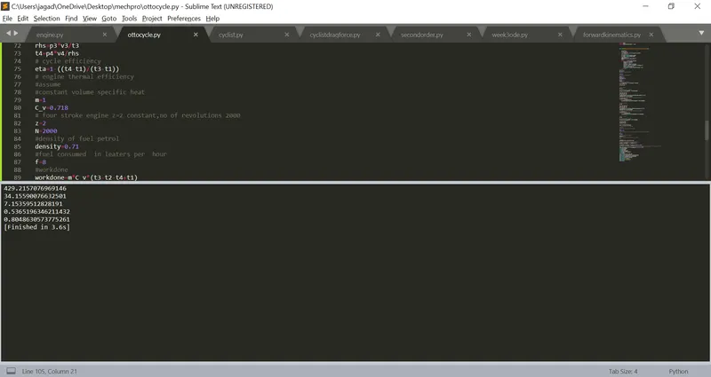
RESULTS:
cycle efficiency eta=0.80486
thermal efficiency=0.5365
PV plot:
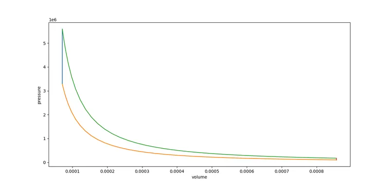
From the above graph we can see that the plot for pv from the program is same as that of the thearatical.
Applications of Otto Cycle:
The applications of Otto Cycle are as follows.
- The Otto cycle was essential for the modern world where it can provide energy for most of the transportation.
- You can see the variety of automobiles seen on the road which uses the Otto Cycle to convert gasoline into motion i.e. Chemical Energy--> Heat Energy-->Mechanical Energy.