Week 3 - Solving second order ODEs

Second order function:

The given second order pendulum equation is

`(d^2theta)/dt^2+b/m*(d theta)/dt+g/l*sin theta=0`

let theta0=theta1 =angular displacement

`(d theta 1)/dt=theta2`=angular velocity

`(d theta2)/dt=`angular acceleration

up on solving the above equation we get

`(d theta1)/dt=theta2`

`(d theta2)/dt=-{(g/l*sin(theta0))+b/m*theta2 }`

The given input values are:

L=1 metre,

m=1 kg,

b=0.05.

g=9.81 m/s2.

The program is

In this program we first import the modules like

math=for doing maths equations and donating trignometry relations

numpy=for donating arrays and doing maths for arrays

odeint from scipy.integrate= for solving the differential equations (since we are solving the 2nd order differential equation)

before importing odeint we need to install scipy

matplotlib.pyplot =for ploting the curves for given data

Then we assain the given values like l,m,b,g

then we define initial conditions like theta =angular displacement and angular velocity as an array

and the time values from 0 to 20 sec with 150 values in between

for this we use linspace to define it

then as we derived from above equations we define a function for solving the equation

with theta values.

after solving the we store the values as an array in dtheta_dt

dtheta_dt array has two values first coiumn as angular velocity

and second value as angular acceleration

After calculating the values are assained to theta and they are stored as theta values

we use the first value for making an animation

we use v to store the first values of the theta

the v value is the angle with which the pendulum is moving

we use for loop to get the plot for each and every theta value.

The pendulum consists of fixed point,string and a bob

fixed point:It is considered as an initial value

let us consider the initial values (x,y)=(0.0)

string and bob

let (x1,y1) be the posistion of the bob

x1=l*sin(theta)

y1=-l*cos(theta)

we define the bob by using the plt and mark command as defined inthe program

string is the length between the bob and the fixed point and these are defined as in the program.

we plot for each theta value and save the file

we use imagemagick to make an animation

import math
import numpy as np
from scipy.integrate import odeint
import matplotlib.pyplot as plt
def model(theta,t,b,g,l,m):
	theta1=theta[0]
	theta2=theta[1]
	dtheta1_dt=theta2
	dtheta2_dt=(-(b/m)*theta2-(g/l)*math.sin(theta1))
	dtheta_dt=[dtheta1_dt,dtheta2_dt]
	return dtheta_dt
b=0.05
g=9.81
l=1
m=1
#initial conditions
theta_0=[0,3]
#time points
t=np.linspace(0,20,150)
#solve ode
theta=odeint(model,theta_0,t,args=(b,g,l,m))
	#plot results
"""plt.plot(t,theta[:,0],'b-')
plt.plot(t,theta[:,1],'r--')
plt.xlabel('time')
plt.ylabel('plot')
plt.show()"""
#annimation
v=theta[:,0]
x=0
y=0
ct=1

for ang in v:
	x1=l*math.sin(ang)
	y1=-l*math.cos(ang)
	pendulum=str(ct)+'.png'
	ct=ct+1
	plt.figure()
	plt.plot(0,0)
	plt.plot([0,x1],[0,y1])
	plt.plot(x1,y1,'bo',14)
	plt.xlim(-1.2,1.2)
	plt.ylim(-1.2,0)
	plt.savefig(pendulum)
	

RESULTS:

plots for angular velocity and angular acceleration are

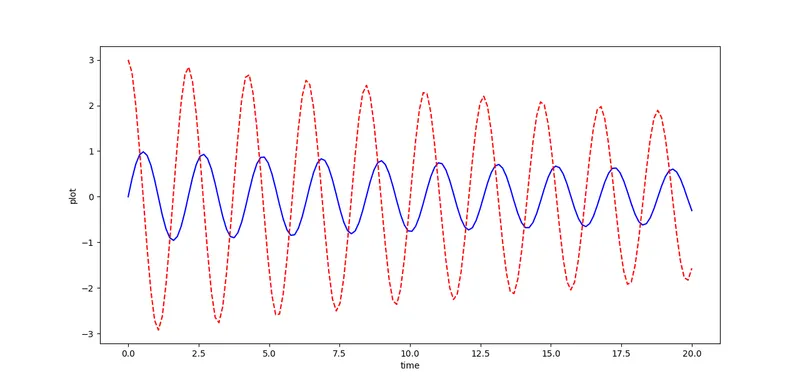
from the graph we can see the velocity and acceleration are decreasing due to the damping factor and they are uniform

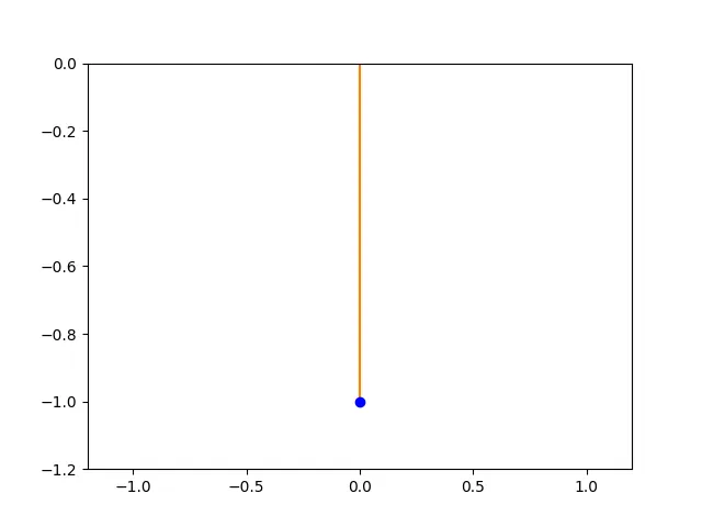
animation link:

https://youtu.be/ZefcC4_Wkj4

problems faced :

Not able to define the theta value properly for posistion of the bob

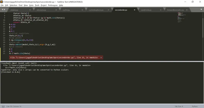
IT had showed me error of size array

first i had defined an value array to store the first values of the theta

Then i used for loop for each value to create an plot as shown in the program

Then i am able to get the plots and saved them and created an animation.