Week 5 - Curve fitting
Curve fitting :
capturing the trend in the data by assigning a single function across the entire range is called an curve fitting.
There are different types of curve fittings here we discuss mainly about linear and polynomial curve fittings.
Linear curve fitting or linear regression:
The basic equation is `f(x)=a*x+b`
here we need to find the a and b coefficients to get the better fit the data in the equation
polynomial curve fitting or higher order polnomial functions:
The basic equation for an nth order polynomial is
`f(x)=a0+a1*x^1+a2*x^2+a3*x^3+........+an*x^n`
where a0,a1,a2... an are coefficients need to find to get the better fit of data in the equation.
We use python to get the values of coefficients .
In python we use curve fit command that is imported from the scipy module.
The command is
Popt,Pcov =curve_fit(function,atributes)
where
Popt are the best fit parameters that are coefficients for the assumed function
Pcov variable contains the covarance matrix.Which indicates the uncertainities and correlations between parameters.
Example with the given data for curve fitting:
The given data is temperature and the specific heats(cp) we need to get a curve that better fits the given data such that we can assume the further specific heats for a given temperature.
The program in python is:
import math
import numpy as np
import matplotlib.pyplot as plt
from scipy.optimize import curve_fit
#defining a function
def linear(t,a,b):
	return a*t+b
def quadratic(t,a,b,c):
	return a*pow(t,2)+b*t+c
def cubic(t,a,b,c,d):
	return a*pow(t,3)+b*pow(t,2)+c*t+d
def polynomial(t,a,b,c,d,e):
	return a*pow(t,4)+b*pow(t,3)+c*pow(t,2)+d*t+e
def quintic(t,a,b,c,d,e,f):
	return a*pow(t,5)+b*pow(t,4)+c*pow(t,3)+d*pow(t,2)+e*t+f
def seventh(t,a,b,c,d,e,f,g,h):
	return a*pow(t,7)+b*pow(t,6)+c*pow(t,5)+d*pow(t,4)+e*pow(t,3)+f*pow(t,2)+g*t+h
#reading the file
def read_file():
	temperature=[]
	cp=[]
	for line in open('data','r'):
		values=line.split(',')
		temperature.append(float(values[0]))
		cp.append(float(values[1]))
	return [temperature,cp]


#Main program
#linear
temperature,cp=read_file()
popt,pcov=curve_fit(linear,temperature,cp)
fit_cp1=linear(np.array(temperature),*popt)
s=np.sum(cp)
l=np.size(cp)
m=s/l
error1=pow((fit_cp1-cp),2)
sse1=sum(error1)
#print(sse1)
deviation1=fit_cp1-m
ssr1=sum(pow(deviation1,2))
#print(ssr1)
rmse1=pow((sse1/l),0.5)
#print(rmse1)
sst1=sse1+ssr1
Rsquare1=ssr1/sst1
print(Rsquare1)
#quadratic
popt,pcov=curve_fit(quadratic,temperature,cp)
fit_cp2=quadratic(np.array(temperature),*popt)
error2=pow((fit_cp2-cp),2)
sse2=sum(error2)
#print(sse2)
deviation2=fit_cp2-m
ssr2=sum(pow(deviation2,2))
#print(ssr2)
rmse2=pow((sse2/l),0.5)
#print(rmse2)
sst2=sse2+ssr2
Rsquare2=ssr2/sst2
print(Rsquare2)
#polynomial
popt,pcov=curve_fit(cubic,temperature,cp)
fit_cp3=cubic(np.array(temperature),*popt)
error3=pow((fit_cp3-cp),2)
sse3=sum(error3)
#print(sse3)
deviation3=fit_cp3-m
ssr3=sum(pow(deviation3,2))
#print(ssr3)
rmse3=pow((sse3/l),0.5)
#print(rmse3)
sst3=sse3+ssr3
Rsquare3=ssr3/sst3
print(Rsquare3)
#polynomial
popt,pcov=curve_fit(polynomial,temperature,cp)
fit_cp4=polynomial(np.array(temperature),*popt)
error4=pow((fit_cp4-cp),2)
sse4=sum(error4)
#print(sse4)
deviation4=fit_cp4-m
ssr4=sum(pow(deviation4,2))
#print(ssr4)
rmse4=pow((sse4/l),0.5)
#print(rmse4)
sst4=sse4+ssr4
Rsquare4=ssr4/sst4
print(Rsquare4)
#fifth order polynomial
popt,pcov=curve_fit(quintic,temperature,cp)
fit_cp5=quintic(np.array(temperature),*popt)
error5=(fit_cp5-cp)
sse5=sum(error5)
#print(sse5)
deviation5=fit_cp5-m
ssr5=sum(pow(deviation5,2))
#print(ssr5)
rmse5=pow((sse5/l),0.5)
#print(rmse5)
sst5=sse5+ssr5
Rsquare5=ssr5/sst5
print(Rsquare5)
#seventh order polynomial
popt,pcov=curve_fit(seventh,temperature,cp)
fit_cp7=seventh(np.array(temperature),*popt)
error7=pow((fit_cp7-cp),2)
sse7=sum(error7)
#print(sse7)
deviation7=fit_cp7-m
ssr7=sum(pow(deviation7,2))
#print(ssr7)
rmse7=pow((sse7/l),0.5)
#print(rmse7)
sst7=sse7+ssr7
Rsquare7=ssr7/sst7
print(Rsquare7)
#ploting the graphs
plt.plot(temperature,cp,color="red",linewidth=3)
plt.plot(temperature,fit_cp1,color="blue",linewidth=3)
plt.plot(temperature,fit_cp2,color="green",linewidth=3)
plt.plot(temperature,fit_cp3,color="yellow",linewidth=3)
plt.plot(temperature,fit_cp4,color="black",linewidth=3)
plt.plot(temperature,fit_cp5,color="orange",linewidth=3)
plt.plot(temperature,fit_cp7,color="gray",linewidth=3)
plt.xlabel('temperature')
plt.ylabel('spectific heats_cp')
plt.legend(['real','linear','quadratic','cubic','polynomial','quintic','seventh'])
plt.show()
Explanation:
1.In the above program we had imported curve_fit from scipy module
2.Then we had assumed and defined an linear and polynomial functions to fit the given data .
3.We had read the data of the given file and store the values in the respective temperature and specific heats (cp)
4.The we used the curvefit command to calculate the coefficients of the assumed function from the given data .
5.Here Popt will give the optimum variables for thr assume function.
6.Pcov gives the covariance matrix .The diagonal elements are the variances. They tell us how likely the parameter is to vary.
7. *Popt in the program means using all the variables that are obtained in the Popt output.
8.The np.array(temperature) uses all the temperature values to calculate the specific heats at all the temperatures.
RESULTS:
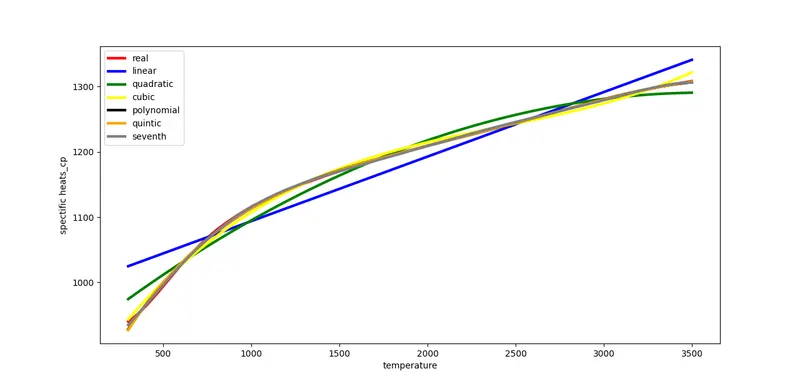
From the above results we can say that the cubic function and above degree polynomial functions better fits the given data.
From the graphs we can say that the higher order polynomial functions give the better fit to the given data.
EMPIRICALLY:
After using graphical methods to evaluate the goodness of fit, you should examine the goodness of fit statistics. The Curve Fitting Toolbox supports these goodness of fit statistics for parametric models:
- The sum of squares due to error (SSE)
- R-square
- Root mean squared error (RMSE)
Sum of Squares Due to Error. This statistic measures the total deviation of the response values from the fit to the response values. It is also called the summed square of residuals and is usually labeled as SSE.
A value closer to 0 indicates a better fit.
R-Square. This statistic measures how successful the fit is in explaining the variation of the data. Put another way, R-square is the square of the correlation between the response values and the predicted response values. It is also called the square of the multiple correlation coefficient and the coefficient of multiple determination.
R-square is defined as the ratio of the sum of squares of the regression (SSR) and the total sum of squares (SST). SSR is defined a
SST is also called the sum of squares about the mean, and is defined a
where SST = SSR + SSE. Given these definitions, R-square is expressed as
R-square can take on any value between 0 and 1, with a value closer to 1 indicating a better fit. For example, an R2 value of 0.8234 means that the fit explains 82.34% of the total variation in the data about the average
If you increase the number of fitted coefficients in your model, R-square might increase although the fit may not improve.
Root Mean Squared Error. This statistic is also known as the fit standard error and the standard error of the regression
where MSE is the mean square error or the residual mean square
A RMSE value closer to 0 indicates a better fit.
RESULTS:
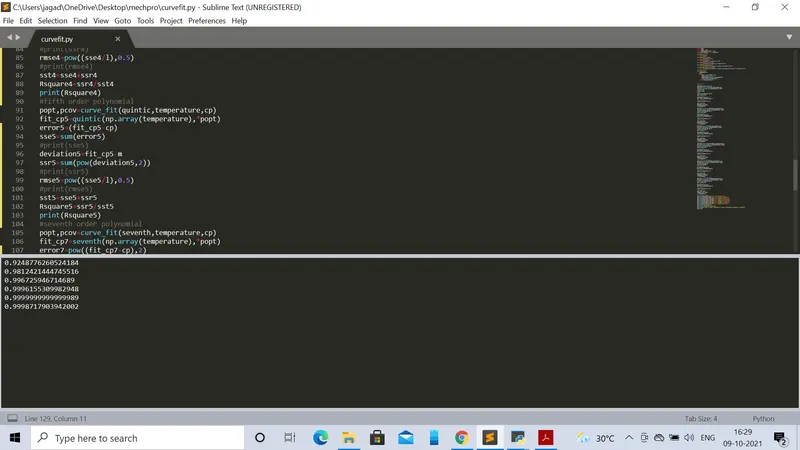
The Rsquare value for 5th degree polynomial that is quintic function has better curve fitting values.since it is close to 1.when compare to other function.
CONCLUSION:
Hence empirically we can say that the polynomial function with 5th order is better fit in the given data.