Week 6: Conjugate Heat Transfer Simulation

Aim:

To Setup a flow simulation through a pipe with inlet Reynolds number 7,000 using K-Epsilon Turbulence modelling and Supercycling method.

To perform Grid dependence test using 3 grids and find out value of Y+ and to show convergence of temperature to a particular value in each case.

To study Effect of supercycle stage interval by setting up with supercyle stage interval to 0.01,0.02 and 0.03.

Conjugate Heat Transfer (CHT)

The exchange of thermal energy between the two physical bodies is called as the phenomenon of heat transfer. The rate of heat transferred is directy proportional to temperature difference between the bodies. Conjugate Heat Transfer(CHT) is a process which involves temperature variations in solids and fluids due to the thermal interaction between them. In solids conduction dominates, whereas in fluids ususally convectiondominates. When we have multiple modes of heat transfer i.e. conduction /convection, it is called as CHT. Forced convection is the most common way to achieve high heat transfer rate. In some applications, the performances are further improved by combining convection with phase change.

Y+

Y+ is a dimensionaless quantity that can be used to understand the kind of mesh. The behaviour of the flow near the wall is a complicated phenomenon and to distinguish the different regions near the wall the concept of wall has been formulated. Thus Y+ is a dimensionless quantity, and it is distance from the wall which is measured in terms of viscous lengths. If we intend to resolve the effects near the wall i.e., in the viscous sub layer then the size of the mesh size should be small and dense enough near the wall so that almost all the effects are captured. But in some cases if the wall effects are negligible then in that case the mesh need not to be dense or small near the wall i.e., coarse mesh would work.

Super - Cycling Method

Super-cycling is a method used by CONVERGE Studio in the cases of conjugate heat transfer problems with a solid and liquid region. Converge solves the fluid heat transfer using the Navier-stokes energy equation and solid heat transfer using the solid heat equation. The scenario in CHT case is that both solvers cannot run at the same speed since solving in the fluid domain is much faster owing to the time scale difference for heat transfer in liquids compared to solids. This causes problems during the solution given that the solid side solver would not have reached a steady state or convergence in the time the liquid solver does. This is where the concept of super-cycling can be used. The basic idea of super-cycling is that the solver for the fluid domain is paused until the solver for the solid domain converges. This pausing is done in intervals that can be set by the user. Main function of Super-cycling is to speed up the simulation and if the simulation is run without super-cycling, the convergence of the data will take a long time.

Simulation Procedure:

Geometry Creation:

Geometry of pipe is created with the given dimensions. Two cyclinders - one inner and other outer are created. Hit diagnosis, if there are any normal orientation errors, go to Transform> normal > Select any triangle and hit apply.

Now go to boundary > Flag and select create multiple boundaries.

Geometry clean up and Boundary Flagging:

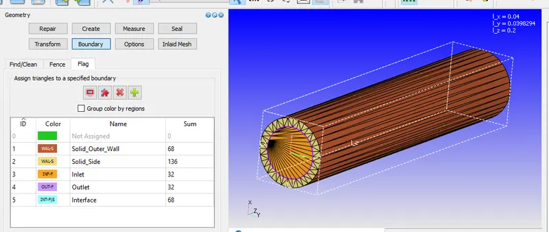
Above figure shows the geometry of the pipe. Geometry is flagged into outer wall and side wall made up of Solid (Aluminium) in which heat flux is generated, inlet, outlet through which fluid flows and Interface between solid and fluid.

Dimensions of Geometry:
Lx = 0.04m

Ly = 0.039m

Lz = 0.2m

Case Setup:

1. Applications type: Time - Based
2. Materials:

Select default values for Gas Simulation and Global Transport Properties and Select Air as Predefined Mixture

select Solid simulation and Add Predefined material - Aluminium in it.

Species : Add N2 and O2 in Gas as Air is the working fluidand Aluminium in Solid

3.Initial Condition and Events:

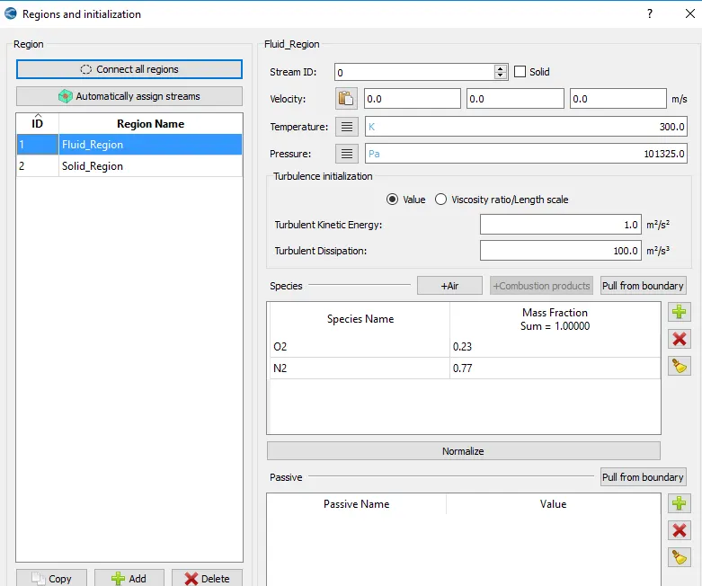
Two regions are need to be added. Add first region as Fluid_region in regions and Initialisation and intialise species value with below mass fraction

O2 - 0.23

N2 - 0.77 whose combination makes the Air as the working fluid for simulation.

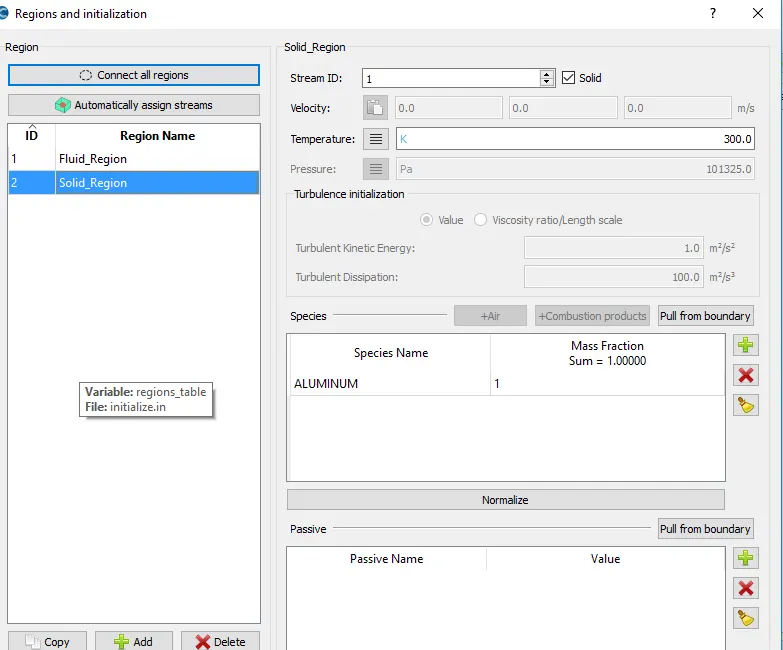
Add second region as Solid_region with stream ID- 1 and Check in the Solid box as the material is solid and add Aluminium with mass fraction 1 for species.

1. Boundary Conditions:

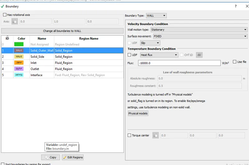
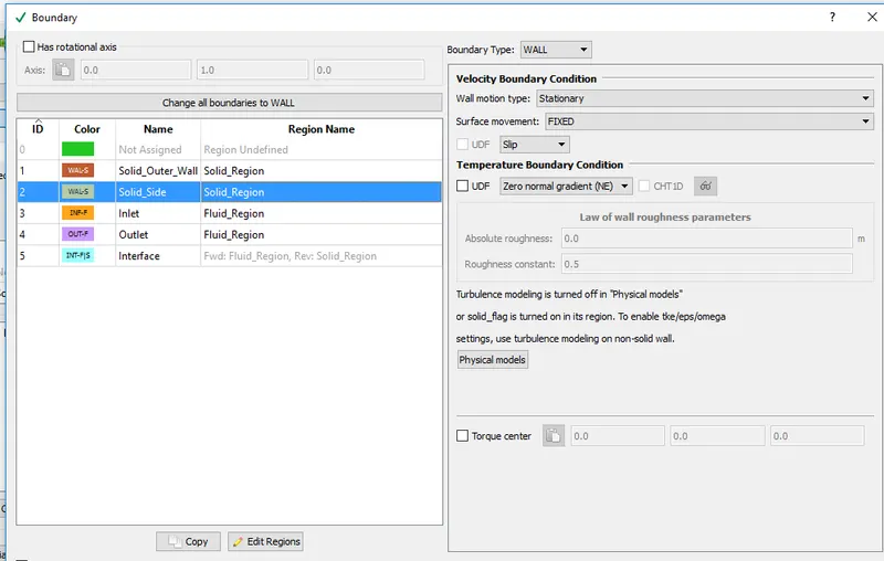
Outer solid wall

Since it is made up of solid select solid region in the Region name.

Heat flux of 10000 W/m2 is generated at this wall. Negative sign indicates heat is flowing into the system.

Solid Side wall:

Since it is made up of solid select solid region in the Region name.

Inlet

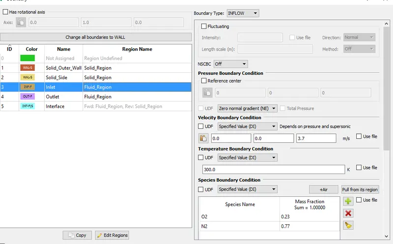
Boundary type - INFLOW.

Pressure - Zero Normal Gradient (Neumann BC)

Calculatiing Inlet Velocity

`Re = (rho * V * d)/(mu)`

Where Re is the Reynolds number and is 7000

`rho` is the density of fluid, here it is air and its value is 1.161 `(kg)/m^3`

V is the velocity of fluid and is to be calculated

`mu`is the Dynamoic Viscosity of Air and is `1.85 * 10^(-5)`

d is the inner diameter of pipe(through which fluid flows) and is 0.03m

So `V = (Re * mu)/ (rho * d)`

`V = (7000 * 1.85*10^(-5))/ (1.161 * 0.03)`

which gives V = 3.71 m/s

So Inlet Velocity is 3.7 m/s along z-axis

Temperature - 300 K

Species - N2 = 0.77 and O2 = 0.23

Region is Fluid_region

Outlet

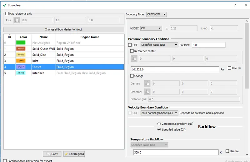
Boundary type - OUTFLOW.

Pressure - 101325 Pa

Velocity - Zero Normal Gradient (Neumann BC)

Temperature - 300 K

Species - N2 = 0.77 and O2 = 0.23

Also mention O2 and N2 species for Backflow ( if it occurs due to adverse pressure)

Interface:

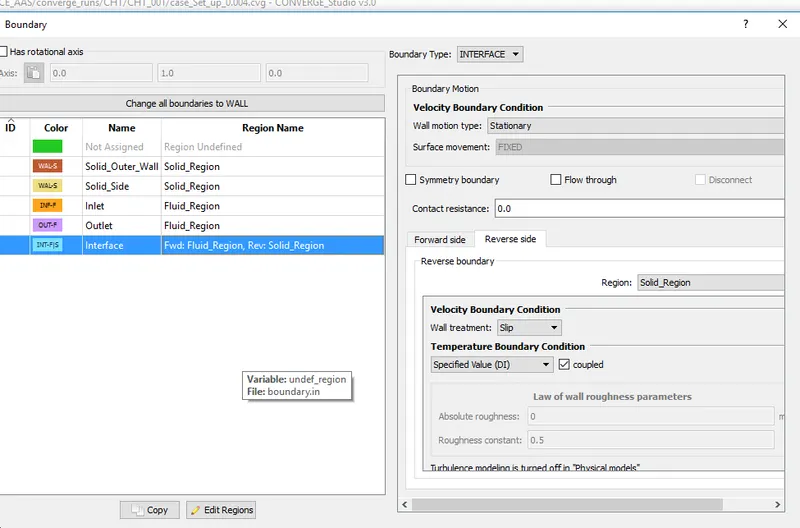
It is the interface between solid and fluid. So it has two sides forward and reverse. Forward side is the side along which the normal of the triangles of interface is facing.Reverse is the opposite of it. Approprite bcs are provided at these two sides. Here forward side is the fluid_region and reverse is the Solid_region.

Froward Side:

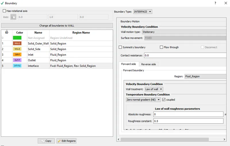
Reverse_Side:

5. Simulation Parameters:

Run parameters:

Solver : Transient

Simulation mode: Full hydrodynamic

Turn off use shared memory.

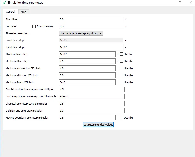
Simulation Time Parameters:

Start time - 0 seconds

End time - 0.5 seconds

Intial time step : 1e-7 s

Minimum time step:1e-7 s

Maximum Time step: 1 s

Maximum convection CFL limit: 1

Leave the rest as Default values.

And the same is shown in below figure

Solver Parameters:

N-S solver Scheme - PISO

N-S Solver Type - Density Based

6. Physical Models:

Turbulence model : RNG k -`epsilon` in RANS

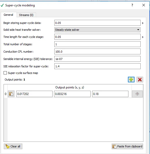
Add super-cycling

Mention the parametrs like begin time for stroing super cycle data and time length for each cycle stage.

Time intervals of 0.01s, 0.02s and 0.03 sec for a particular mesh size are simulated.

Select a point inside the domain to moniter the heat/temperature value.

7. Grid Control :

Base grid : dx=0.004m dy= 0.004m and dz = 0.004 m and grid dependency test is performed by using mesh size of 3mm and 2mm in other cases.

Output/Post-processing

In post variable selection, under Species tab, add N2, O2 and Aluminium in mass fraction box.

In the Output generation tab under Output files, select Boundaries only for Wall Output as this will dump wall averaged output data which is very much important for any external aerodynamic simulations.

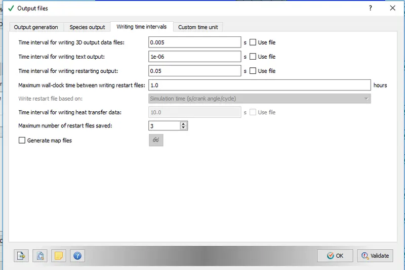
In output files, under Writing time intervals tab, in order to obtain 100 3D output files to capture the results accurately, time interval for writing 3D output data files and restarting files is specified as 0.005 sec and 0.05 sec since the end time is 0.5 seconds. 1e-6 sec is provided to time interval for writing text output so outputs are obtained at each cycle of simulation.

Now Export All these input files to a directory. Open CYGWIN, navigate to the directory where all these folders are saved and run the following command ;

mpiexec.exe -n 4 converge.exe restricted </dev/null> logfile_006 &

which runs the simulation with 4 processors using converge executable and outputs are dumped into a file called logfile_006 with job being ran in backend.

Outputs/Post -Processing:

Post processing is performed in the paraview software using the group files with ..vtm extension created in the post processor of Converge

Case - 1: Mesh size - 4mm

Mesh:

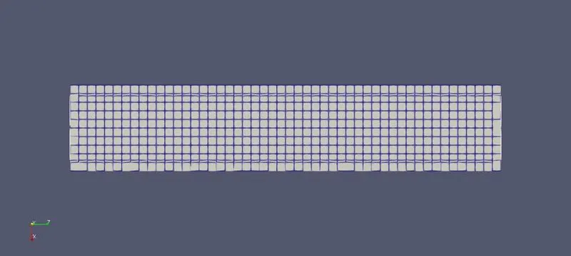
Mesh is coarse and cell size are quite large

Velocity Contour:

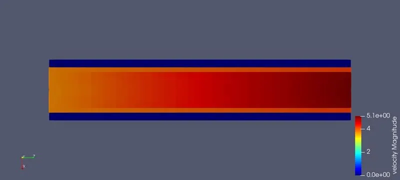
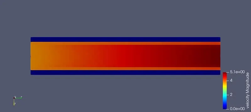
Velocity increases from initial value of 3.7m/s to 5.1m/s. Velcoity is 0 in the solid region (Outer wall) as there is no flow of fluid

Y+:

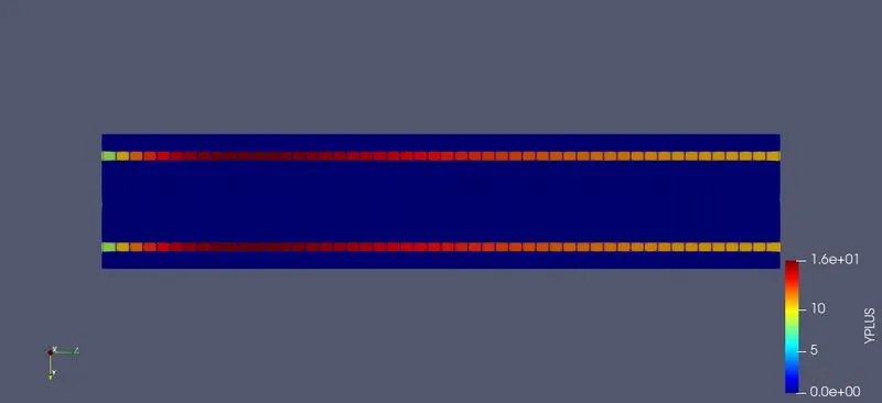
value of Y+ is 16 which means the first cells are in Transition region. Value of Y+ below 10 incidates the cells in the boundary layer are in Sub viscous layer and cell size are small

Temperature Contour:

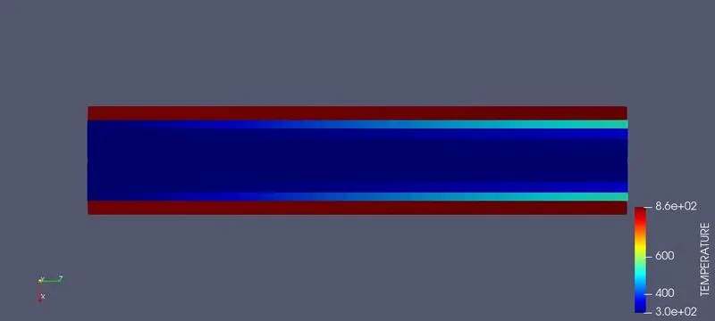
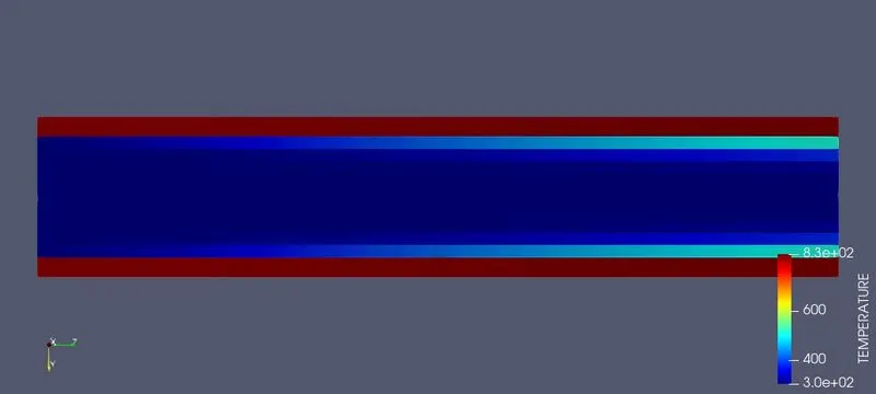
Temperature is higher in the solid region since heat is generated in this region. Due to the transfer of heat from Solid to fluid, temperatre distribution inside the pipe can be visualised. Temperature at outlet is quite larger than the inlet.

Mean Temperature:

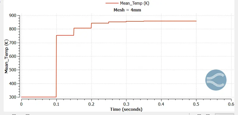
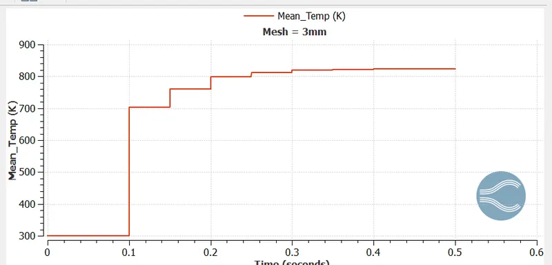
We can see the increase in temperature in stages. Due to heat transfer from solid, we can see rise in the temperature as the simulation progresses.

Cell count:

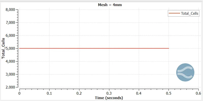
Since the size of cell is large, number of cells in the domain is less and is around 5000.

Average Temperature at Outlet:

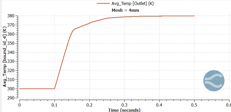
Temperature at the outlet rises from initial value of 300K to 380K and converges at the end of the simulation at 0.4 seconds.

Temperature Animation:

Case - 2: Mesh size - 3mm

Mesh:

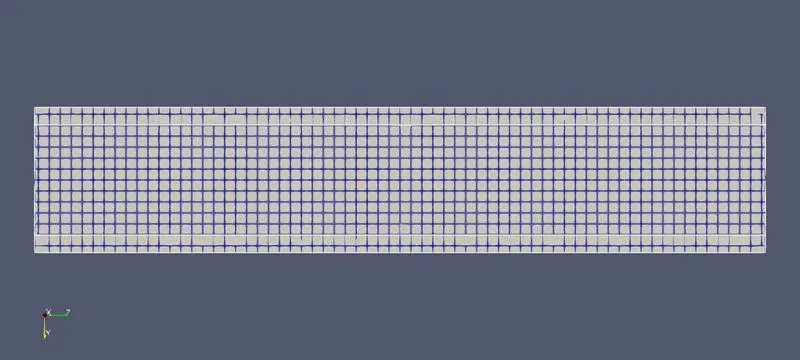
We can see the decrease in the size of the cell due to reduced mesh size of 3mm.

Velocity Contour:

Y+:

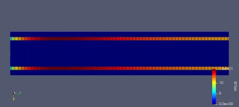
value of Y+ is 16 which means the first cells are in Transition region. Value of Y+ below 10 incidates the cells in the boundary layer are in Sub viscous layer and cell size are small

Temperature Contour:

Mean Temperature:

Cell count:

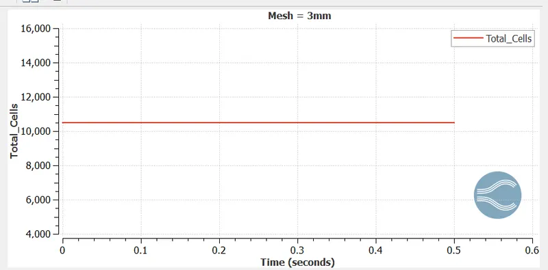
Since the cell size is quite small, we can see the rise in the number of cells in the domain and is around 11000

Average Temperature at Outlet:

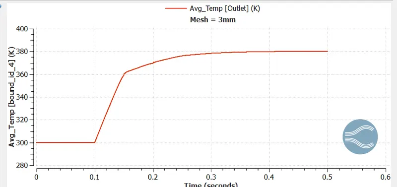
Temperature at the outlet rises from initial value of 300K to 380K and converges by the end of the simulation at 0.4 seconds.

Temperature Animation:

Case - 3: Mesh size - 2mm

Mesh:

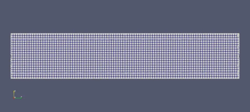
Due the reduction in the mesh size, we can see the finer mesh and increase in the number of cells and reduction in cell size. Results are accurately captured with finer mesh but simulation time increases for the finer mesh

Velocity Contour:

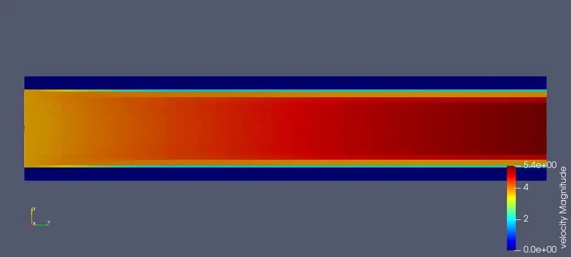
Distribution of velocity across the geometry is more clear due to the reduced mesh size. Maximum velocity is around 5.4m/s and simualtion was initialised with inlet velocity of 3.7m/s

Y+:

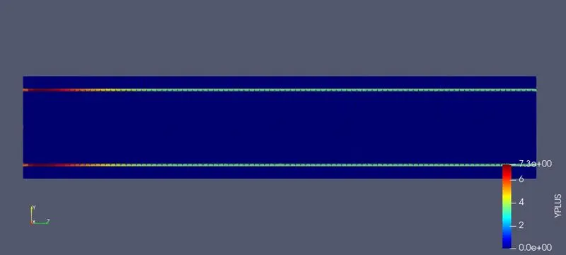
Since the cell size is smaller, first set of cells in the voundary layer are in sub- viscous layer. This is evident from the value of Y+ as it is below 10. Value of Y+ between 10 to 30 indicates that the first cell are in transition region and value of Y+ above 30 indicates cells are in turbulent region. If the aim is to capture the accurate results with viscous effects, cell size in trhe domain should be smaller so that Y+ value is below 30 and it makes the mesh finer and increases simulation time.

Temperature Contour:

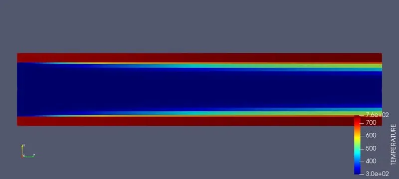
Maximum value fo temperature is 760K and it is lower than that of above cases. Due to smaller cell size results captured are accurate. Temperature in equal in the entire solid region (Outer wall).

Mean Temperature:

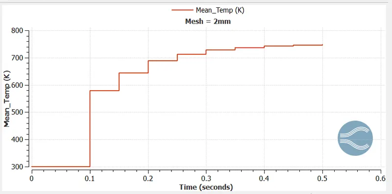
Mean temperature is increasing in stages and it is around 750K

Cell count:

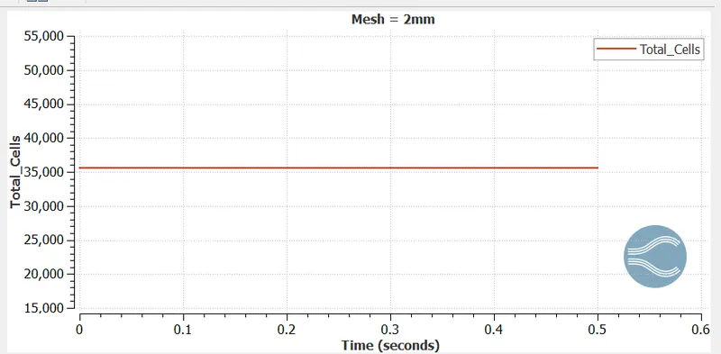
Due to reduced mesh size, number of cells is higher in this case and is around 36000.

Average Temperature at Outlet:

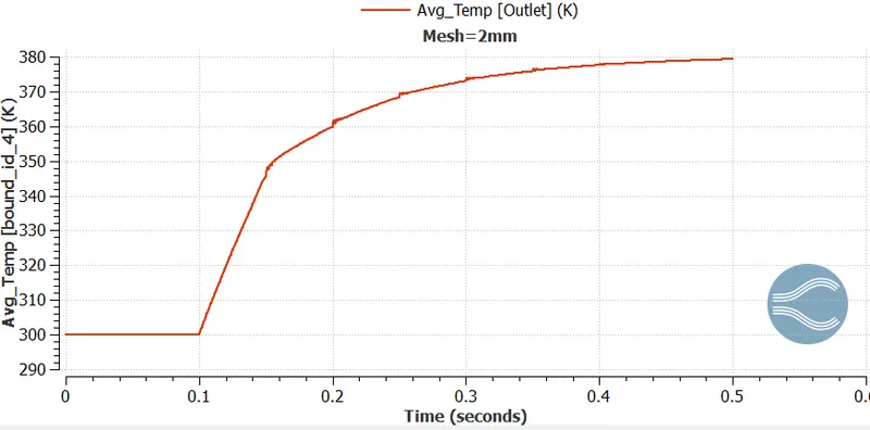
Average temperature is not yet coverged at outlet for the given simulation time but it is almost convegring and reaching a value of 380K.

Temperature Animation:

Effect of Super Cycling Interval

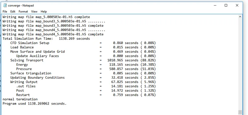
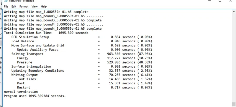
Simulation is carried out for super cycling interval of 0.01s, 0.02s and 0.03 sec with 3mm base nesh size in all three cases and time taken for simulation in each case is compared

Super Cycling Interval - 0.01 sec and Mesh size - 3mm

Time taken

Super Cycling Interval - 0.02 sec and Mesh size - 3mm

Time taken

Super Cycling Interval - 0.03 sec and Mesh size - 3mm

Time taken

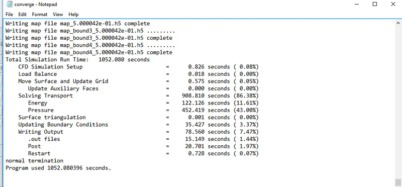
Time taken for simulation with super-cycling interval of 0.03 sec is 1052 sec, 0.02 sec is 1095 sec and 0.01 sec is 1138 seconds.From comparision we can say that simulation time increases a bit as the super cycling interval reduces. But the increase is not much. All simulation with different super cycling intervals are carried out at 3mm mesh size in all three axes.

Conclusion:

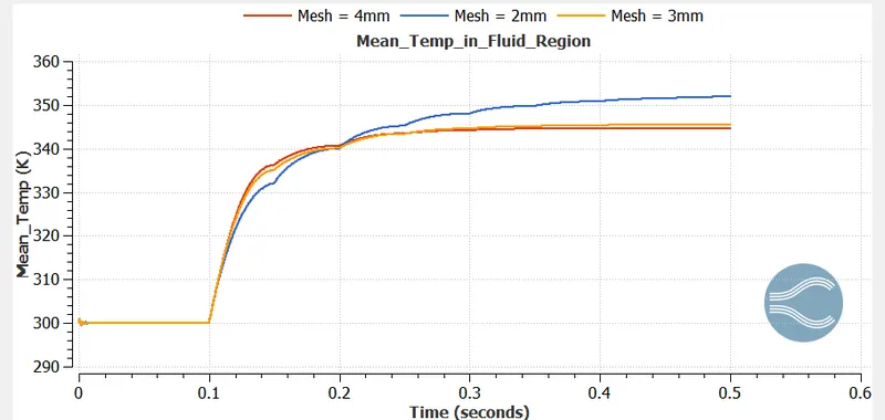
Temperature in Fluid Region:

Temperature in Solid Region:

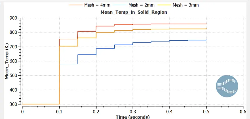
Above figures indicate the mean temperature in fluid and solid region for three different grid Sizes.

We can see that they do not Converge at the same te,perature. The Mean temperature for the Solid is around 800K and the mean temperature for the fluid region is around 350K

The mean temperature in Solid region decreases as the mesh grid size decreases. As the cells are refined further, accurate results are captured.

The mean temperature in Fluid region increases as the mesh grid size decreases. As the cells are refined further, accurate results are captured.

• Studied the effect of super cycling and its importance in reducing simulation time in the cojugate heat transfer problem. Also studied how change in value of super cycling interval changes the simulation time. Studied the heat transfer through solid and fluids.
• Performed grid dependency test with different mesh sizes and its effect on value of Y+. With the smaller mesh size, Y+ value decreases and this value below 10 positions the cells in the viscous sub layer. Value of Y+ below 10 can be obatined with smaller mesh size but the same increases the ssimulation time. Value of temperature is different in different cases of mesh sizes. Results captured with smaller mesh size prove to be accurate although they require higher simulation time.
• Succesfully simulated the conjugate heat transfer problem using CONVERGE and studied the distribution of temperature in pipe.