Week 10: Modeling and Simulation of flow around an Ahmed Body
Aim:
To Create the CAD model of Ahmed body, create virtual wind tunnel around it and Setup a Coarse CFD simulation.
To create an animation of the velocity and pressure distribution on a cutplane that cut the ahmed body model in two symmetric pieces.
To Post process the coarse mesh results and extract the x component of velocity along a line which is perpendicular to the ground plane. Plot velocity at different location using line probes and compare the experimental data with the simulation data.
To Calculate the steady state drag force,lift force value and the drag co-efficient using paraview.
Ahmed Body:
The Ahmed body is a generic car body or a simplified vehicle model created by Ahmed in the 1980s to investigate the behaviour of newly developed turbulence models for complex geometry cases. The airflow around the Ahmed body captures the essential flow features around an automobile and was first defined and characterized in the experimental work of Ahmed. Ahmed body allows us to capture characteristic features that are relevant to bodies in the automobile industry. This model is also used to describe the turbulent flow field around a car-like geometry. Some of the key characteristics which can be obtained from simulating Ahmed's Body are Velocity Magnitude, Pressure Magnitude, Wake region, Drag Force, Lift Force.
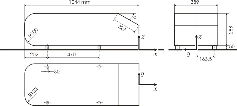
Geometry of Ahmed Body:
Simulation Procedure:
Geometry Creation:
The geomtery dimensions of the Ahmed body are as shown above. Using these dimensions the Ahmed body has been desingned in SOLIDWORKS software and shown below.
Slant angle of `35 ^(0)` used at the rear end since experimental data is available for this angle. All other dimensions of the Ahmed body are made exactly equal to the original geometry.
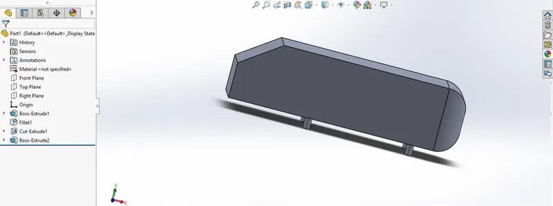
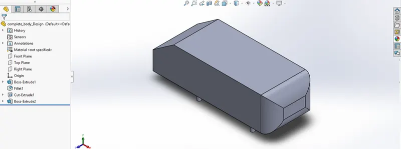
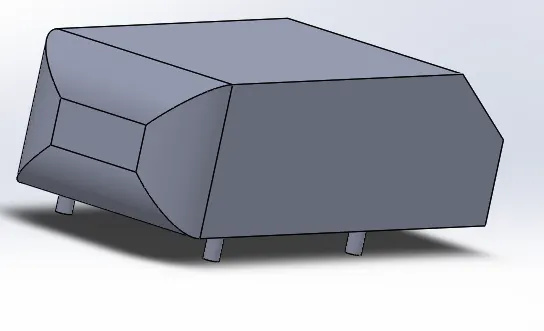
Then save the geometry in the STL format from Solidworks so that it can be compatible with Converge Studio.
Import the file of geometry of the Ahmed Body in STL extension into Converge.
Transform the scale of the aifoil to 0.001 so that the dimensions will be converted to mms.
Now the virtual wind tunnel needs to be created.
Calculating distance required for growth of Boundary Layer:
The boundary layer of thickness 30mm should be developed at a distance of 400mm in front of the Ahmed Body.
So we have formula for approximating boundary layer thickness over a flat and it is given by
`delta = (0.382 ** x)/(Re^(0.2))`
where `delta` is boundary layer thickness and is 30 mm
x is the length of the plate required to develop this boundary layer
Re is the Reynolds number and is given by
`Re = (rho * V * L)/(mu)`
where `rho` is the density of fluid, here it is air and its value is 1.225 `(kg)/m^3`
V is the velocity of fluid and is is considered to be 40m/s flowing from the Inlet.
`mu` is the Dynamoic Viscosity of Air and is `1.85 * 10^(-5)`
L is the length and here it is x which is the length of the flat plate.
So `delta = (0.382 ** x)/((rho*V*x)/(mu))^(0.2)`
`0.03 = (0.382 ** x^(0.8)*(1.85*10^-5)^(0.2))/((1.225*40)^(0.2)`
Solving this yields
`x^(0.8) = (0.03*(1.225*40)^(0.2))/(0.382*(1.85*10^(-5))^(0.2)`
This gives `x =1.667 m`
This means that it requires 1.67m length of the flat plate to develop a boundary layer of thickness 30mm with velocity of air 40m/s.
We need this boundary layer of thickness 30mm at 400 mm in front of Ahmed body. So we need atleast 1.67m + 0.4 m which is 2.07m.
So we will need approximately 2m of length in front of Ahmed body which needs to be no - slip region.
we want a uniform velocity profile at the inlet where there should be no growth of boundary layer to obtain proper free stream,before the region where boundary layer develops, slip boundary condition needs to be provided for a length of 1m (which is the length of AHhmed body, 1*L). In this region of 1m of slip boundary there will be no growth of boundary layer and we will get freestream velocity.
So the total length of Virtual wind tunnel in front of Ahmed body is 2m + 1m = 3m.
The region behind the Ahmed body needs to be between 5* L to 10*L in order to accurately capture wake region. We will consider this length as 6m.
Approximately Total length of wind tunnel is = 3m(Front of Ahmed Body) + + 1m(Length of Ahmed body) + 6m(Rear of Ahmed body) = 10m Approx.
Width of the wind tunnel = 2 * L = 2m
Height of the Wind Tunnel = 2 * L = 2m
So now All dimensions of Virtual wind tunnel are obatined and are given by ( 10 m * 2m * 2m).
Origin is at the bottom right corner( and in ground) of the front face of Ahmed body. From the centre of the front face this point is at a distance of (0.389/2)= 0.1945m. So the vertices of Wind tunnels would be at (0.8055) in negative z axis and 1.1945 in positive z axis.
To create this wind tunnel go to Create > Vertex and create 6 vertices with coordinates (-3,0,-0.8055), (-2,0,-0.8055), (-3,0,1.1945), (-2,0,1.1945), (7,0,-0.8055), (7,0,1.1945).
Now copy these vertices and create at a disatnce 2m away along positive Y-axis. Now all the vertices for wind tunnel of required dimensions are created and is as shown in below figure.
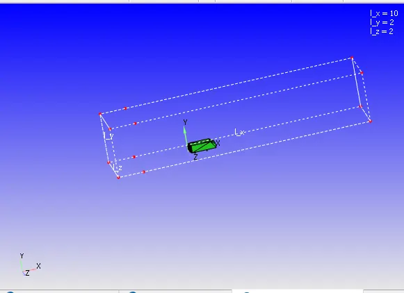
go to repair, Patch these vertices to create faces of wind tunnel with Ahmed body placed on bottom most face. Run diagnosis, and if there are any Normal orientations error, go to Transform > Normal, select any triangle >Apply. Now if there are no errors in the model, our Ahmed body with virtual wind tunnel will be ready for simulation and looks like below.
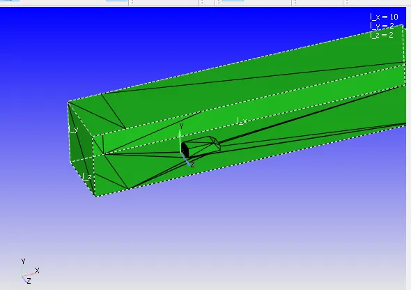
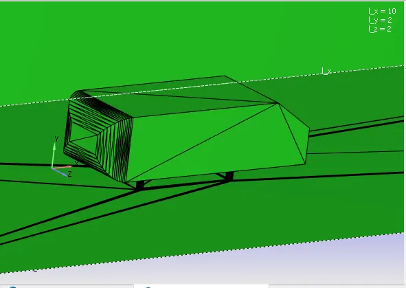
Now go to boundary > Flag and select create multiple boundaries.
Geometry clean up and Boundary Flagging:
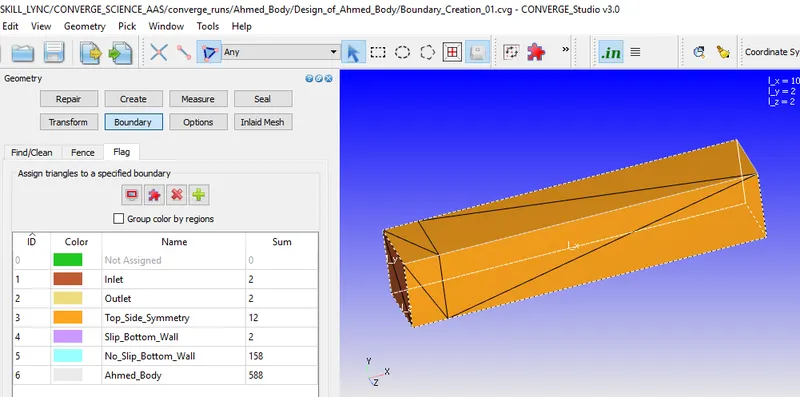
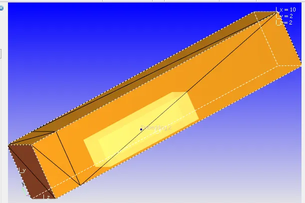
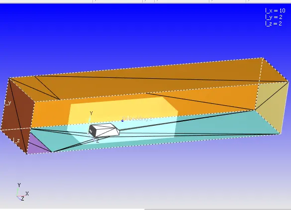
Above figure shows the geometry of the Ahmed Body inside virtual wind tunnel. Geometry is flagged into inlet, outlet, Top and Side Walls which are symmetric about xy plane, Slip bottom wall which is of 1m from Inlet, No slip bottom wall which has boundary layer growth with Ahmed body placed upon it and Ahmed body.
Dimensions of Geometry:
Lx = 10m
Ly = 2m
Lz = 2m
Case Setup:
- Applications type: Time - Based
- Materials:
Select default values for Gas Simulation and Global Transport Properties and Select Air as Predefined Mixture
Species : Add N2 and O2 in Gas
as Air is the working fluid
3.Initial Condition and Events:
Add a region as Volumetric_Region in regions and Initialisation and intialise species value with below mass fraction
O2 - 0.23
N2 - 0.77 whose combination makes the Air as the working fluid for simulation.
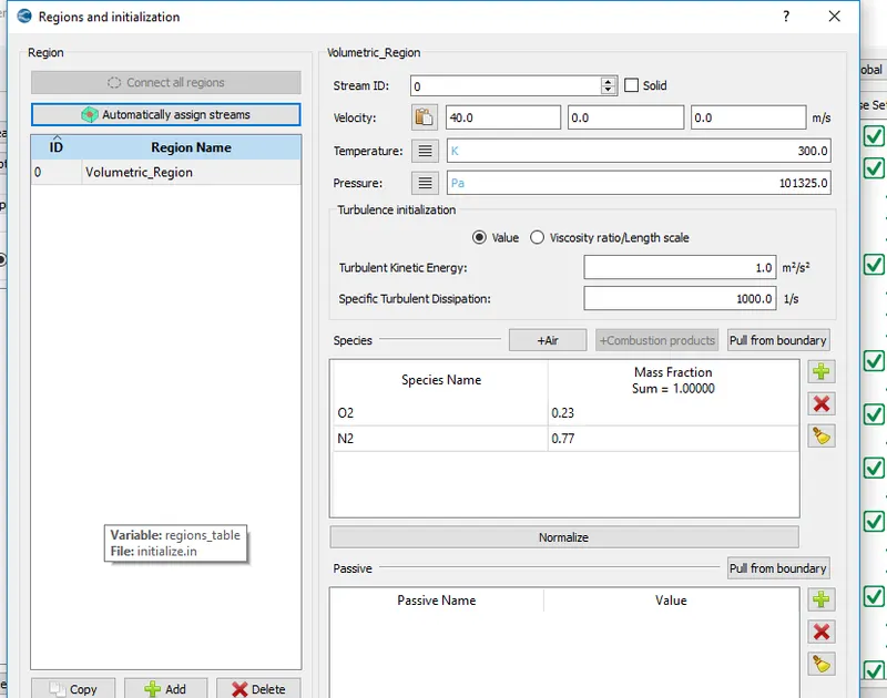
Initialise the Velocity to 40m/s along X-axis at Inlet with 300 K temperature and 1 atm Pressure.
- Boundary Conditions:
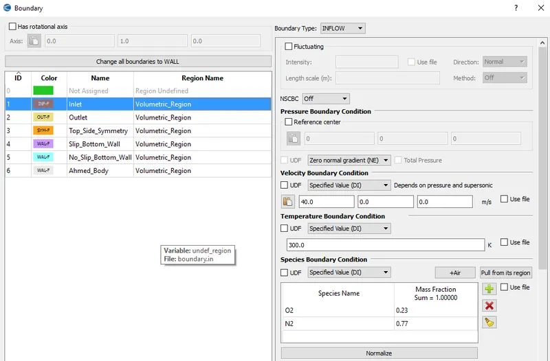
Inlet
Boundary type - INFLOW.
Pressure - Zero Normal Gradient (Neumann BC)
Velocity - 40 m/s along x-axis --- Same value as of regions and Initialisation
Temperature - 300 K
Species - N2 = 0.77 and O2 = 0.23
Outlet
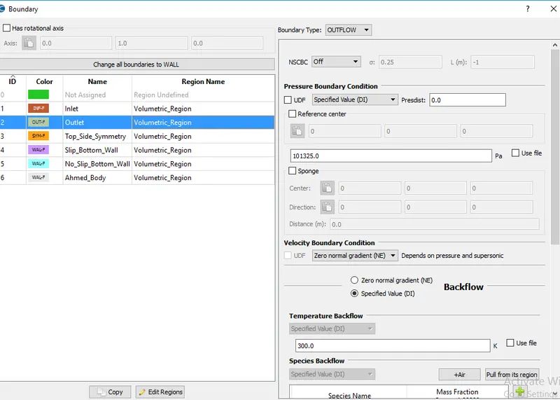
Boundary type - OUTFLOW.
Pressure - 101325 Pa
Velocity - Zero Normal Gradient (Neumann BC)
Temperature - 300 K
Species - N2 = 0.77 and O2 = 0.23
Also mention O2 and N2 species for Backflow ( if it occurs due to adverse pressure)
Top_Side_Symmetry:
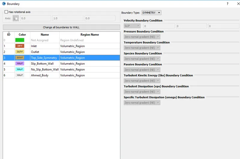
Select boundary type as SYMMETRY boundary type as top and side walls are symmetric about xy plane.
Slip_Bottom_Wall:
Select boundary type as WALL with Stationary wall motion type.
Provide Slip Velocity BC so the inflow velocity will not be changed for some distance (to maintain freestream without Boundary layer formation)
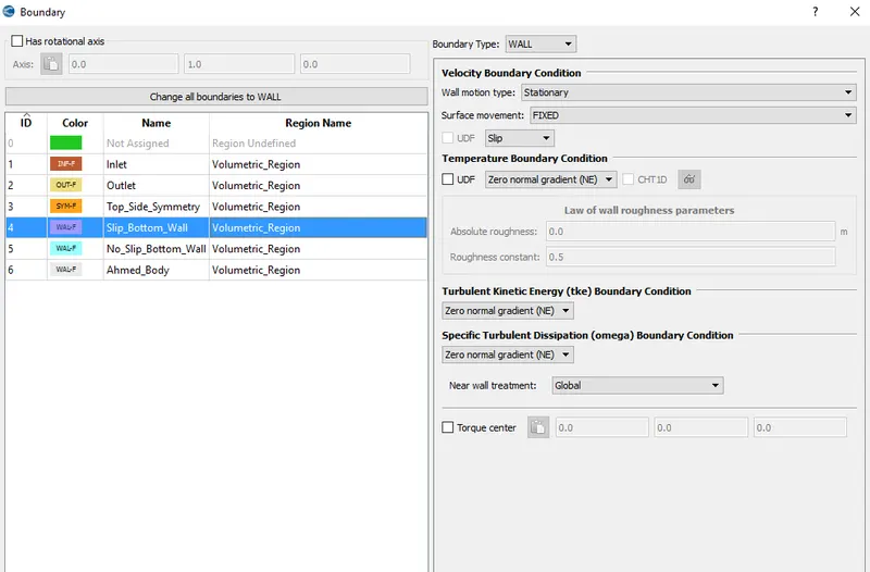
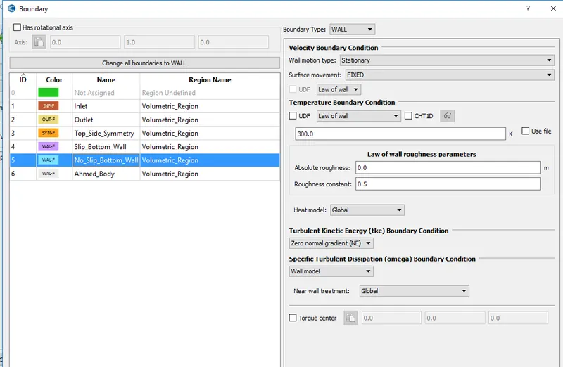
No_Slip_Bottom_Wall:
Select boundary type as WALL with Stationary wall motion type.
Provide law of Wall for Velocity and Temperature BC so the boundary layer starts to develop.
Ahmed Body:
Select boundary type as WALL with Stationary wall motion type.
Provide Law of Wall for Velocity and Temperature BC
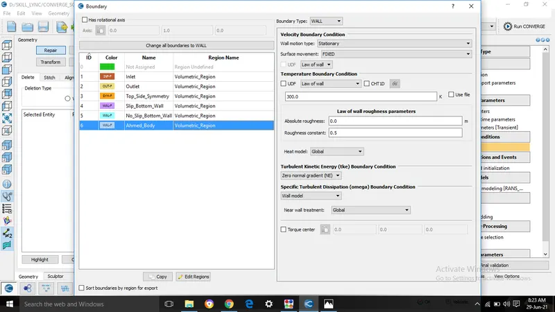
Select Volumetric_Region as Region name for all the boundaries since Volumetric_Region is the region created for the boundaries.
5. Simulation Parameters:
Run parameters:
Solver : Transient
Simulation mode: Full hydrodynamic
Turn off use shared memory.
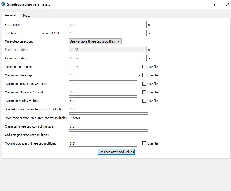
Simulation Time Parameters:
Start time - 0 seconds
Calculating end time for Simulation:
Velocity at the Inlet is 40 m/s .
The Length of the Virtual Wind Tunnel is Lx = 10m. So keeping these values, time needed for the fluid to flow from inlet to outlet will be
`Speed = (distance )/ (time)`
so `time = (distance) / (speed)`
time = 10m / (40m/s) = 0.25 seconds
and this time is called as Flow Through Time and here it is around 0.25 seconds.
Simulation is ran for around 4 times of this flow through time to capture all required values over the Ahmed Body. So
End time =4 * Flow through time = 4 * 0.25 = 1 second and thus it is considered as 1 seconds.
End time - 1 seconds
Intial time step : 1e-7 s
Minimum time step:1e-7 s
Maximum Time step: 1 s
Maximum convection CFL limit: 1
Leave the rest as Default values.
And the same is shown in below figure
Solver Parameters:
N-S solver Scheme - PISO
N-S Solver Type - Density Based
6. Physical Models:
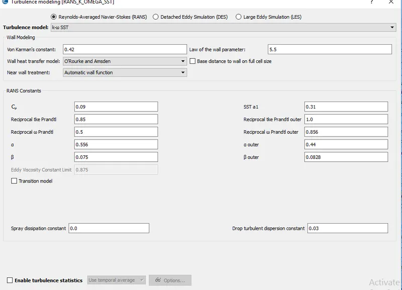
Turbulence model : RNG k -`epsilon` in RANS and K-`omega` SST in RANS and these two models are compared and the best model is selected
Since our aim in the current simulation is to accurately predict the boundary layer growth and velocity , and because the developing boundary layer will tend to separate near Ahmed body( due to a changing pressure gradient and not because of sharp edges or discontinuities in the geometry as in case of Prandtl Meyer Shock Ananlysis Problem) , using low-Re model is recommended.
Low-Re models are also required for accurate pressure-drop or drag calculations. It is highly recommend to use the Shear Stress Transport (SST) model, although all ω-based models or ε-based models with enhanced wall treatment may be used.
So K-`omega` SST is selected as turbulence model
7. Grid Control :
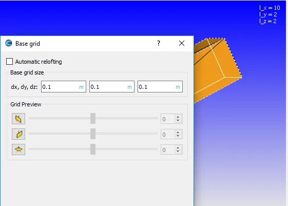
Base grid : dx=0.1m dy= 0.1m and dz = 0.1 m since it is coarse simulation.
Add fixed Embedding in Grid control
Fixed Embedding:
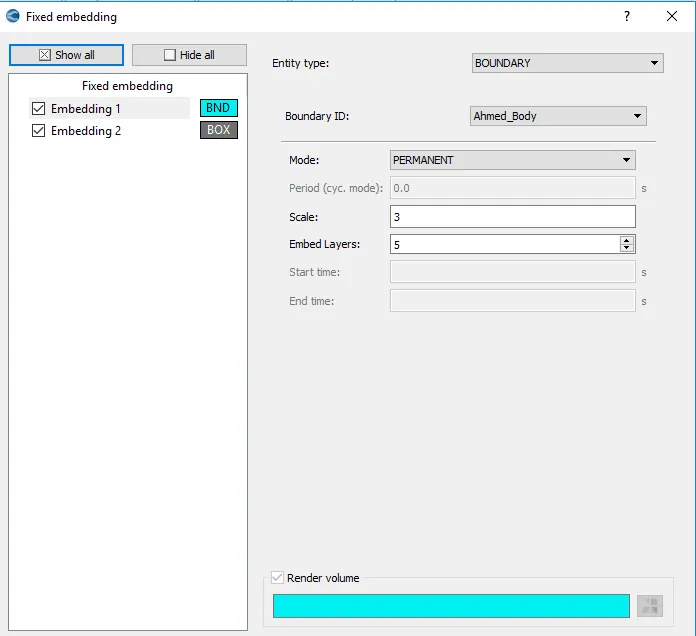
`Embedded Mesh size = (base mesh size) / (2^(SCALE)`
Over the Ahmed body major changes in the flow variables occur. In Order to capture the results accurately over the Ahmed body, fine mesh will be needed with more cells. Making the mesh size smaller in the entire domain is unnecessary as it would increase the simulation time by very large amount. So mesh size is reduced at the Ahmed body alone with the help of a technique called Fixed Embedding of entity type Boundary. Fixed Embedding of Scale of 3 makes the reduces the base mesh size by 8(2^3) times and embedded layers 5 means the mesh size is further reduced by 8 times at the Ahmed body boundary with 5 layers. So fixed embedding is provided at the Ahmed body boundary with Embed layers being 5 and scale of 3 using the PERMANENT mode.
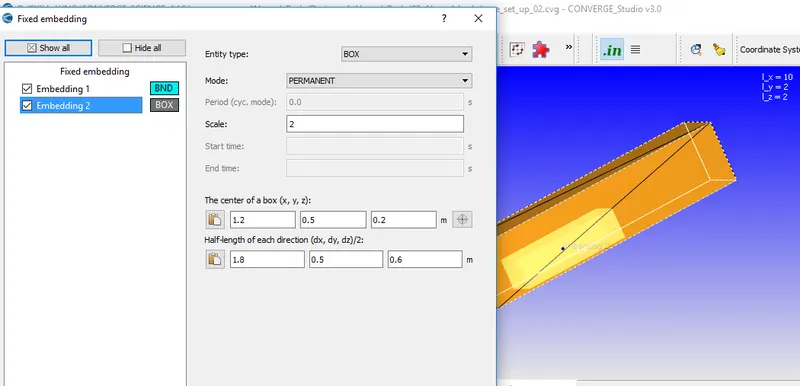
The fixed embediing can also be given for a specified region using Box Entity type. There will be wake region behind ahmed body and in order to capture the reuslts accurately in that region we again need finer mesh. Since there are no walls in that region, a BOX with above mentioned centre and half dimensions along 3 axes are created with scale 2 so that all the cells inside this box region are refined.
Output/Post-processing
In post variable selection, under Species tab, add N2 and O2 in mass fraction box.
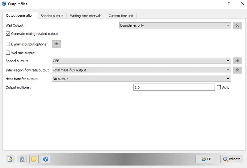
In the Output generation tab under Output files, select Boundaries only for Wall Output as this will dump wall averaged output data which is very much important for any external aerodynamic simulations.
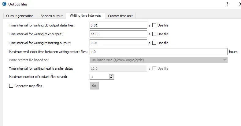
In output files, under Writing time intervals tab, in order to obtain 100 3D output files to capture the results accurately, time interval for writing 3D output data files and restarting files is specified as 0.01 sec and 0.05 sec since the end time is 1 seconds. 1e-5 sec is provided to time interval for writing text output so outputs are obtained at each cycle of simulation.
Finalised case set up with different boundaries, Virual wind tunnel, Ahmed body, and Box embedding can be seen below.
Now Export All these input files to a directory. Open CYGWIN, navigate to the directory where all these folders are saved and run the following command ;
mpiexec.exe -n 4 converge.exe restricted logfile_006 &
which runs the simulation with 4 processors using converge executable and outputs are dumped into a file called logfile_006 with job being ran in backend.
Outputs/Post -Processing:
Post processing is performed in the paraview software using the group files with ..vtm extension created in the post processor of Converge
Mesh:
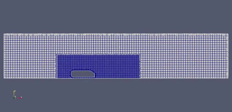
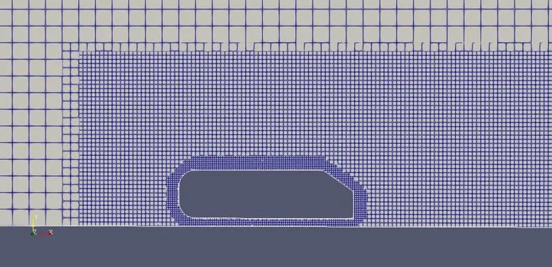
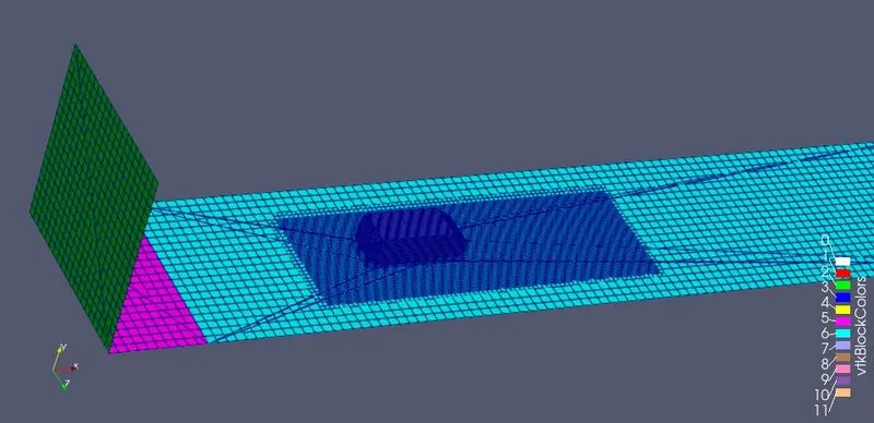
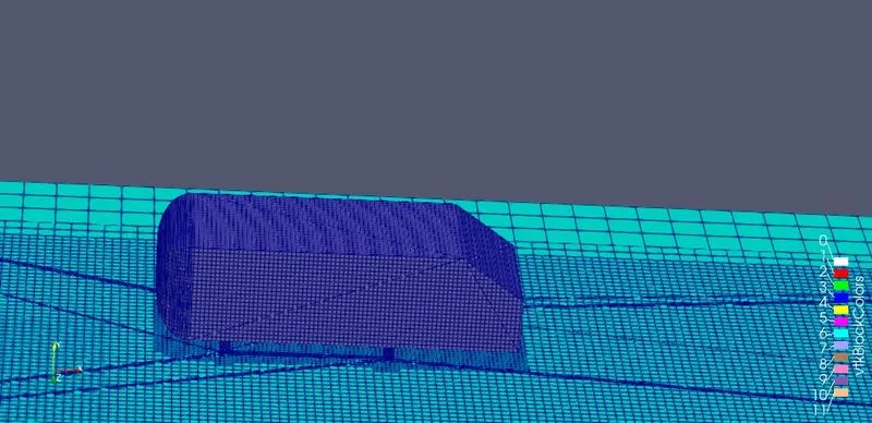
We can see the base mesh being refined at diffrent levels. Since two types of fix embedding are given with scale 2 and 3 for box and Ahmed body respectively we can see refinement in those regions with specified number of layers and the results are captured better in these regions dur to small mesh size and more number of mesh cells.
Pressure Contour:
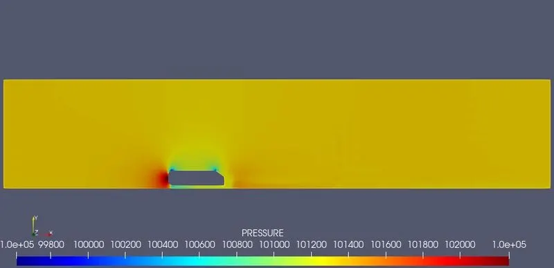
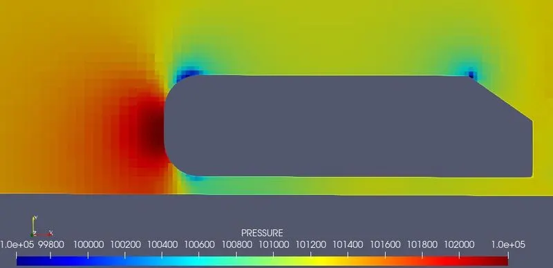
We can see the rise in the pressure in front face of the Ahmed body. When flow hits this surface, the kinetic energy the flow is converted into pressure since the flow comes to rest when it hits this surface and this point is also known as stagnation point where there is increase in the pressure and drop of velocity.
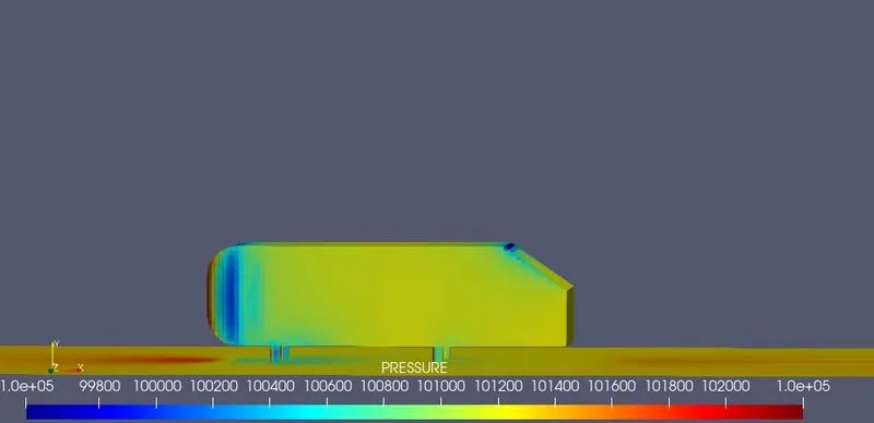
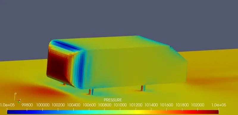
On the edges of the Ahmed body we can see the lesser pressure because velocity is higher on this surfaces.
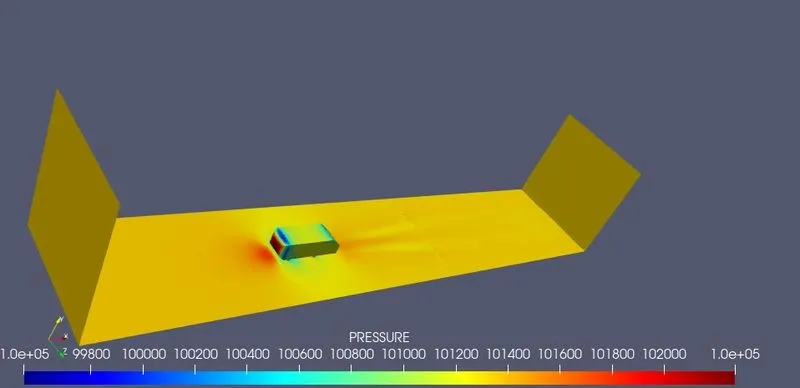
We can see the lesser pressure in the region behind the Ahmed body. This region is characterised by low pressure and low velocity and known as Wake region. Since there is slant design at the rear, when fluid flow past on this, there are lesser fluids flowing in the wake region. If the pressure is lot lesser in the wake region, that would result in recirculation of fluid.
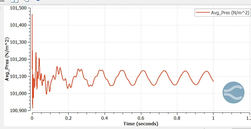
Average Pressure:
Velocity Contour:
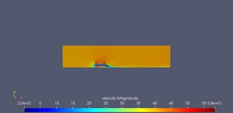
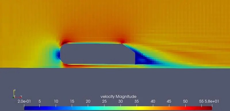
We can also see the velocity being minimum on the front face of Ahmed body. This is the region where flow almost comes to rest leading to reduced velocity and increased pressure as this region is stagnation point.
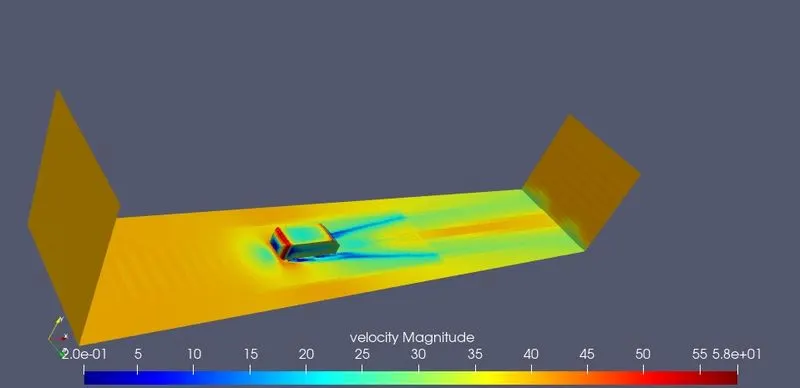
On the edge like surfaces of Ahmed body the velocity is higher. The higher the velocity, lower the pressure.
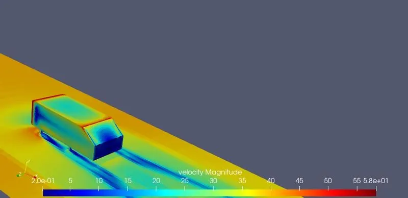
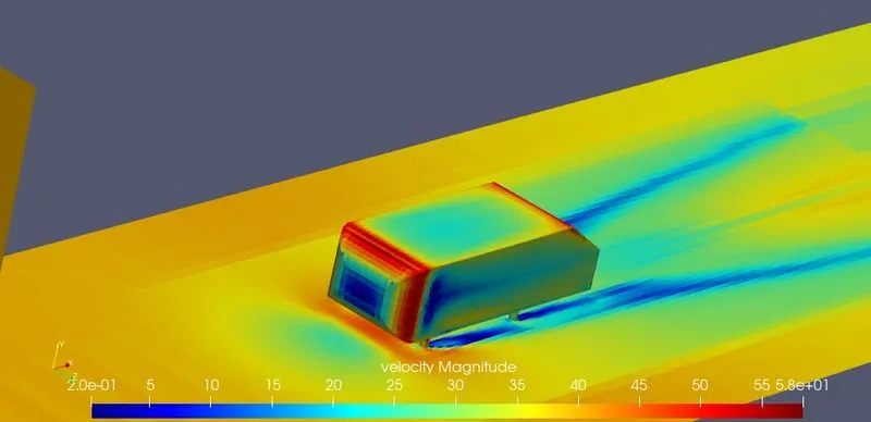
We can see the velocity is lesser in the region behind the Ahmed body. This is the wake region and is characterised by low velocity and low pressure. Due to the slant angle of Ahmed body in the rear, the fluid after flowing past it, makes an angle with horizontal and doesnt able to flow in the region behind ahmed body making wake region with low velocity and low pressure.
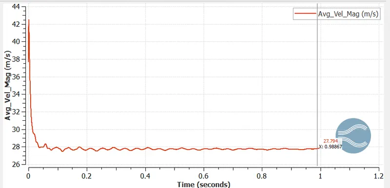
Average Velocity:
Pressure Force along X-axis:
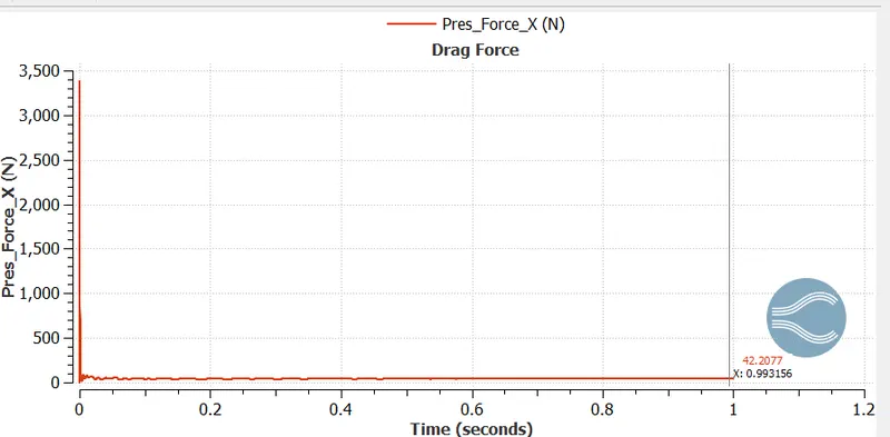
These values are retrived from the folder Wall output - boundaries only - folders which have the average values of the output data around the selected boundary. IN this case we have selected the Ahmed body boundary so we have the average values of the flow variables around Ahmed body.
The Average Pressure force along X-axis is nothing but the drag force as The component parallel to the relative freestream velocity is called Drag. Here the value is 42.2N. So drag coeffeiceint can be calculated from equation for Drag, D which is given by `D = (1/2 * rho * V^(2)* S * Cd)`
So coeffiecient of Drag, `Cd =(2 * D)/(rho * V^(2)*S)`
where D = 42.2 N
rho = 1.225 kg/m3 is density of Air
V = 40 m/s is the freestream velocity flowing from the inlet
S = It is the frontal area and is approximately (0.288*0.389) = 0.112 m^2.
So `Cd = (2 **42.2)/(1.225 **40^(2)**0.112)`
Cd = 0.384
Pressure force along Y-axis:
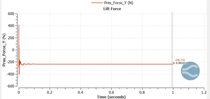
The Average Pressure force along Y-axis is nothing but the lift force as The component of this force perpendicular to the relative freestream velocity is called Lift. The equation for Lift,L is given by `L = (1/2 * rho * V^(2)* S * Cl)`
So coeffiecient of Lift, `Cl =(2 * L)/(rho * V^(2)*S)`
where L = -236.73N
So `Cl = (2 ** (-236.73))/(1.225 **40^(2)**0.112)`
Cl = -2.15
Negative sign indicates force is in opposite direction to the positive Y-axis.
Calculating Drag Force from PARAVIEW:
Search Extract Block in Filter and Extract Ahmed body.
Then Extract the Surface and Generate Surface normals. Now in the Calculator, select (Pressure * Normal_X) in drop down menu of Scalars, and finally in the integrate variables select Attribute as Cell data and the below shown data will be displayed with Drag force = (Pressure * Normal_X) = 40.8623 N
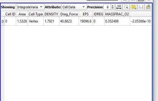
With this value of Drag force we can calculate the drag coefficient just as the above.
`D = (1/2 * rho * V^(2)* S * Cd)`
So coeffiecient if Drag, `Cd =(2 * D)/(rho * V^(2)*S)`
where D = 40.863 N
rho = 1.225 kg/m3 is density of Air
V = 40 m/s is the freestream velocity flowing from the inlet
S = It is the frontal area and is approximately (0.288*0.389) = 0.112 m^2.
So `Cd = (2 **40.863)/(1.225 **40^(2)**0.112)`
Cd = 0.372 from PARAVIEW.
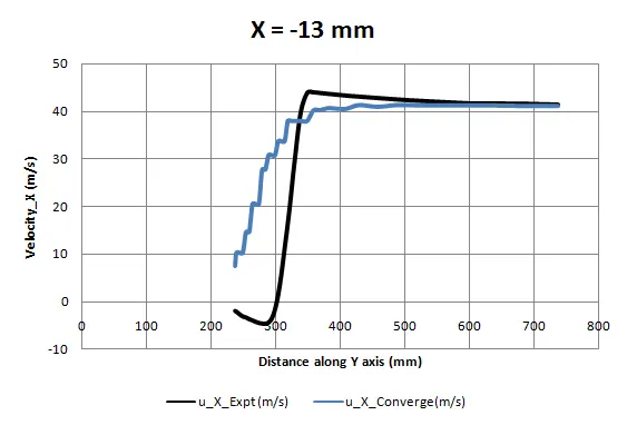
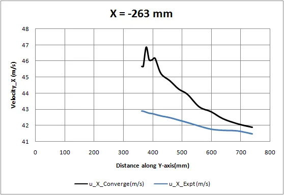
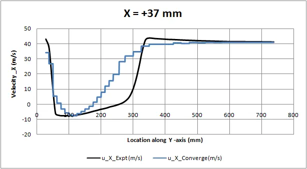
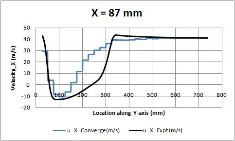
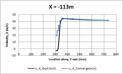
Comparision of simulation results with Experimental data using line probes at different locations of X : Validation
The Values of experimental data is provided and we need to compare those result with the data obtained from our simulation at different points.
Since the origin of experimental data is at the centre line of the back of the Ahmed body and origin for our simulation is at the front bottom part, the distance are need to exactly manipulated before in order to obtain simulation values at exact locations where experimental data is available. Value of 1044mm which is length of the Ahmed body is added to all the given distances along x-axis
1.At x= -13mm
2.At x = -263 mm
3.At x = +37 mm
4.At X= +87 mm
5.At X= -113 mm
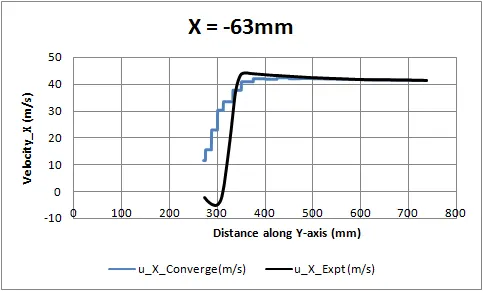
6.At X= -63 mm
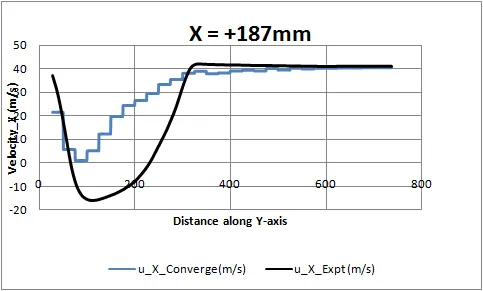
7.At X= +187 mm
8. At X= +137 mm
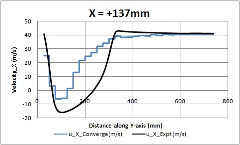
We can see some amount of error between the experimental and simulation data. This is because our simulation is ran with coarser mesh and the cell sizes are big. The error would be reduced by making use of smaller cells but it would require lot more computational resource. But the current results obtained from our simulation are satisfatory.
Plots which are having positive x axis are just behind the Ahmed body which is wake region charcaterised by low pressure and drop in velocity.
Normalised Plot:
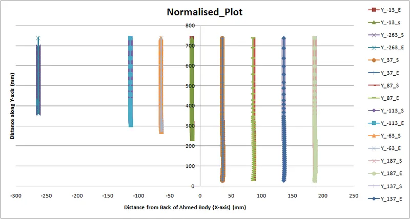
Normalised Velocity = (Amplification_Factor) * `(Velocity)/(Max Velocity)` along Y-axis at any distance along x-axis. Origin indicates the back most point centre of the Ahmed body. The plots are almost identical because the Maximum velocity in bith cases are almost same.
E symbolises the Experimental Data
S indicates the Simulation Data obtained form Converge in above normalised plot.
Streamlines around Ahmed body:
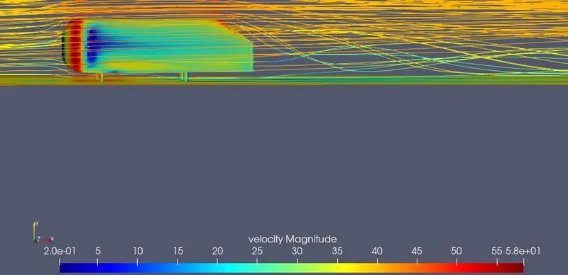
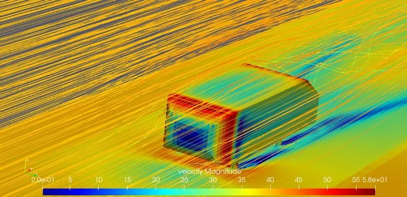
Streamlines replicates the flow pattern of Fluid in Virtual wind tunnel and around Ahmed body.
Animation of Pressure:
Animation of Velocity:
Conclusion:
The velocity magnitude is normalized so as to compare the results obtained by 2 or more line plots simultaneously on a single plot.
For Negative x values, the error between Experimental and Simulation results are quite less. This is due to the smaller mesh in those regions obtained from Fixed embedding. Error can be reduced for positive x values too by reducing mesh size. This comes with disadvantage of increased requirement for computational energy if cell number is increased.
Validation of results has performed by comparing simulation results with Experimental data using line probes at different locations of X and values are satisfactory for this coarser simulation.
The variation of Pressure and Velocity contours in the entire wind tunnel is studied. The major variation takes place at Ahmed body. So as to capture the results accurately around Ahmed body, mesh size is reduced and cells are made finer around it using Fixed embedding technique.
To get the freestream and uniform velocity, slip region is created in bottom face for around 1m. No slip region iof 2m is created so as to develop boundary layer and Ahmed body is placed in no slip region ( or law of Wall) so it is in viscous region and develops viscous forces. To get the flow in wake region, wind tunnel is extended for 6m behind Ahmed body.
The pressure is higher at the front surface of Ahmed body where flow contacts and comes to rest. The velocity is lower at this region and is called as stagnation point.
Both pressure and velocity are lower in the region behind the Ahmed body where there is less amount of fluid flow and this region is called wake region. Larger pressure drop in this wake region may lead to recirculation zone.
The value of Lift and Drag force is obtained from Converge and Paraview and coefficient of Lift and Drag are calculated using these values and they are given by
Coefficient of Lift, Cl = -2.15. Negative sign indicates force is along -Y axis and acting upon the body and helping it to stay attached to ground
Coefficient of Drag, Cd = 0.384 from Converge and 0.372 from Paraview