Week 7: Shock tube simulation project
Aim:
To Setup a transient shock tube simulation, To plot the pressure and temperature distribution in the entire domain for entire simulation and To Plot the cell count as a function of time.
Introduction:
A simple shock tube is a tube, usually constructed of metal, in which a gas at low pressure and a gas at high pressure are separated using some form of diaphragm. The diaphragm suddenly bursts open under predetermined conditions to produce a wave propagating through the low pressure section. The shock that eventually forms increases the temperature and pressure of the test gas and induces a flow in the direction of the shock wave.
The low-pressure gas, referred to as the driven gas, is subjected to the shock wave. The high pressure gas is known as the driver gas. The bursting diaphragm produces a series of pressure waves, each increasing the speed of sound behind them, so that they compress into a shock propagating through the driven gas. This shock wave increases the temperature and pressure of the driven gas and induces a flow in the direction of the shock wave but at lower velocity than the lead wave. Simultaneously, a rarefaction wave, referred to as the Prandtl-Meyer wave, travels back in to the driver gas.
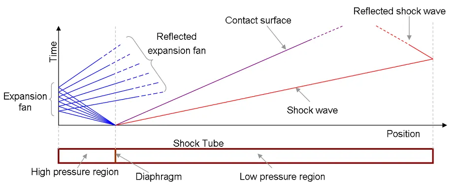
The shock tube used to replicate and direct blast waves at a sensor or a model in order to simulate actual explosions and their effects on a smaller scale. Shock tubes can also be used to study aerodynamic flow under a wide range of temperatures and pressures that are difficult to obtain in other types of testing facilities. Shock tubes are also used to investigate compressible flow phenomena and gas phase combustion reactions(Chemical Kinetics).
A shock wave inside a shock tube may be generated by a small explosion (blast-driven) or by the buildup of high pressures which cause diaphragm to burst and a shock wave to propagate down the shock tube.
Setting up the Simulation in Converge:
Import the geometry file in STL format into the converge environment.
Clean up the geometry, Run diagnosis and if there are any normals orientating outside the geometry, then go to transform, normal and select any triangle and hit apply. All normals should be pointing inwards.
Then go to boundary > Flag and select create multiple boundaries.
Geometry clean up and Boundary Flagging:
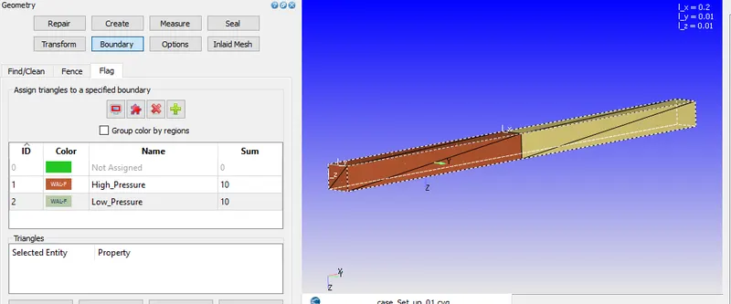
Above figure shows the geometry of the shocktube. Geometry is flagged to two regions named as High Pressure and Low Pressure which will be filled with N2 nd O2 gases respectively in the simulation .
Dimensions of Geometry:
Lx = 0.2m
Ly = 0.01m
Lz = 0.01m
Case Setup:
1. Applications type: Time - Based
2. Materials:
Select default values for Gas Simulation and Global Transport Properties.
Species : Add N2 and O2 in Gas
3. Initial Condition and Events:
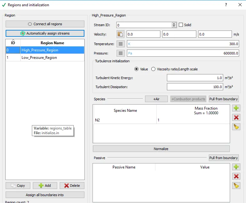
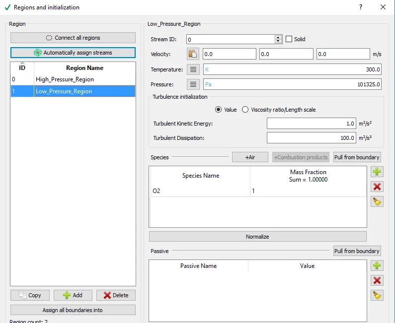
In regions and Initialisation Add two region with stream ID of both being 1.
1st region will be High_Pressure_Region with 300 K and 600000 Pa pressure and contained with N2 of mass fraction 1.
2nd region will be Low_Pressure_Region with 300 K and 1 atm pressure and contained with O2 of mass fraction 1.
4. Boundary Conditions:
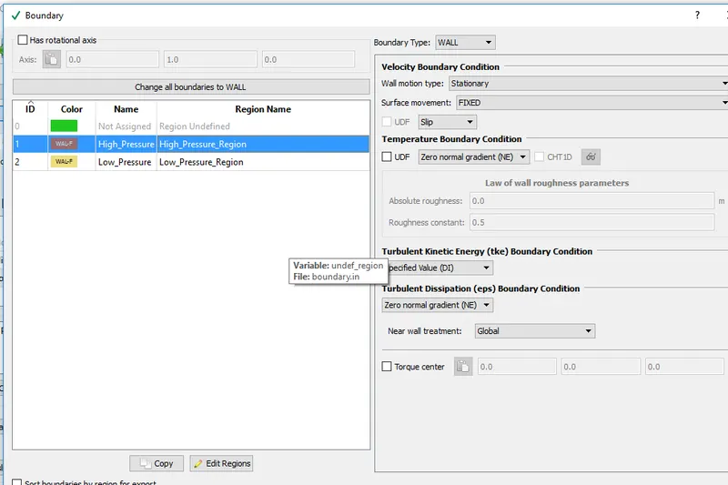
High_Pressure
For high pressure , the boundary type is WALL with slip velocity boundary condition. The whole geometry is made into WALL boundary type filled with N2 and O2 gases initially without inlet and outlet. Select Region name as High_Pressure_Region as this section will be filled with N2 at higher Pressure.
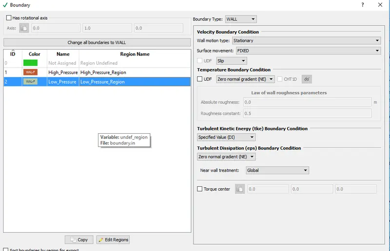
For low pressure, the boundary type is WALL with slip velocity boundary condition. Select Region name as Low_Pressure_Region as this section will be filled with o2 at lesser Pressure.
5. Simulation Parameters:
Run parameters:
Solver : Transient solver
Simulation mode: Full hydrodynamic
Turn off use shared memory and turn on steady state monitor Misc tab.
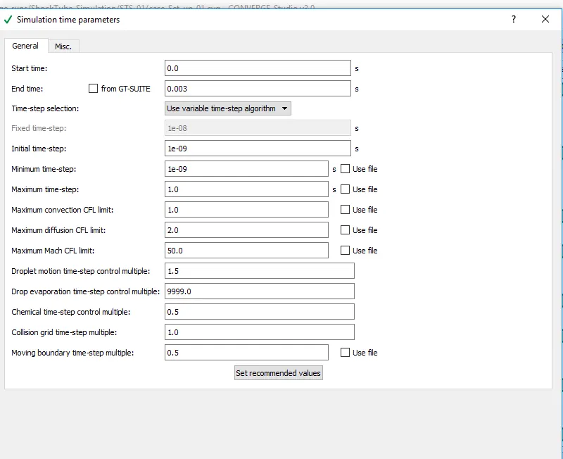
Simulation Time Parameters:
Start time - 0 sec
End time - 0.003 secs
Intial time step : 1e-9 s
Minimum time step: 1e-9 s
Maximum Time step: 1 s
Maximum convection CFL limit: 1
Leave the rest as Default values.
Solver Parameters:
NS solver Scheme - PISO
NS Solver Type - Denisty Based Steady
6. Physical Models:
Turbulence model : RNG k -`epsilon` in RANS
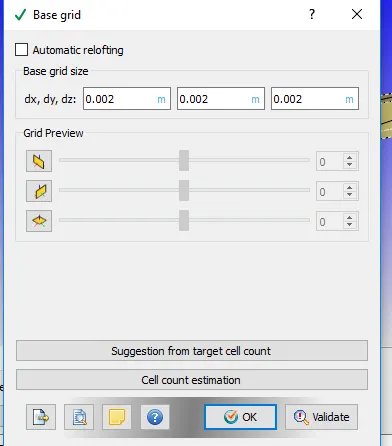
7. Grid Control :
Base grid : dx=dy=dx = 0.002 m
Adaptive Mesh Refinement:
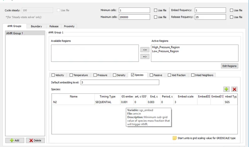
We need finer mesh to capture the accurate values of the varibales. In this current problem, the values will vary in a region where there is contact between N2 and O2. So in order to capture the accurate results there we need smaller and finer mesh in that region. Making the mesh size smaller in the whole geometry will lead to large number of cells and it is unnecesary. So we will make use of a technique called Adaptive Mesh Refinement. The technique makes the geomtery finer only in certain region where the given conditions satisfies capturing the accurate results with lesser number of cells and also this region wil be varying throughout simulation. In this problem we make use of Species varibale which refines the mesh based on the mass fraction of species between the cells. Sub-Grid Scale criterion is used for Embed type with embedding scale of 3.
The given value of sub-grid criterion is 0.001. Given 0.001 is the minimum sub grid value of species mass fraction that wikk trigger Adaptive Mesh refinement. the refined mesh size will be
`REFINED Mesh Size = (Base Mesh)/ (2^(EMBEDD LEVEL))`
Events:
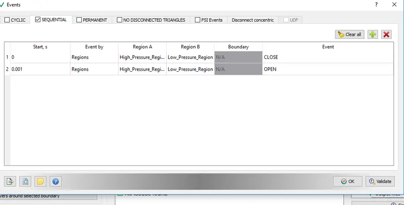
In order to simulate the bursting of the diaphargm virtually we make use of something called Events in Initial Condition and Events.
The two regions (High Pressure and Low pressure Regions) remain CLOSE for first 0.001 sec and it is made OPEN after which with will lead to mixing of two gases in these regions creating a effect of bursting of diaphargm. After this we can see the effect of mixing of gases in the simulation. Select SEQUENTIAL in Events.
8. Output/Post-processing
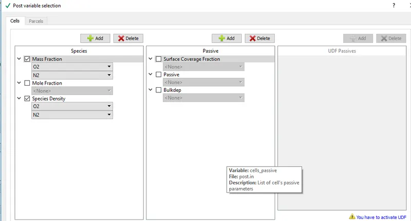
In post variable selection, under SPecies tab, add N2 and O2 in mass fraction box.
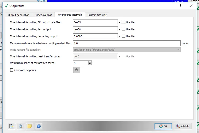
In output files, under Writing time intervals tab, specify 3e-5 sec as time interval for writing 3D output data files to get 100 output files and 3-4 as time interval for restarting files.
Export All these input files to a directory. Open CYGWIN, navigate to the directory where all these folders are saved and run the following command ;
mpiexec.exe -n 4 converge.exe restricted logfile_006 &
which runs the simulation with 4 processors using converge executable and outputs are dumped into a file called logfile_006 with job being ran in backend.
Outputs/Post -Processing:
Post processing is performed in the paraview software using the group files with ..vtm extension created in the post processor of Converge
Mesh:
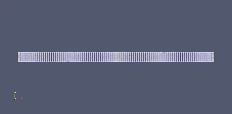
The mesh on the entire domain in the initial stage.
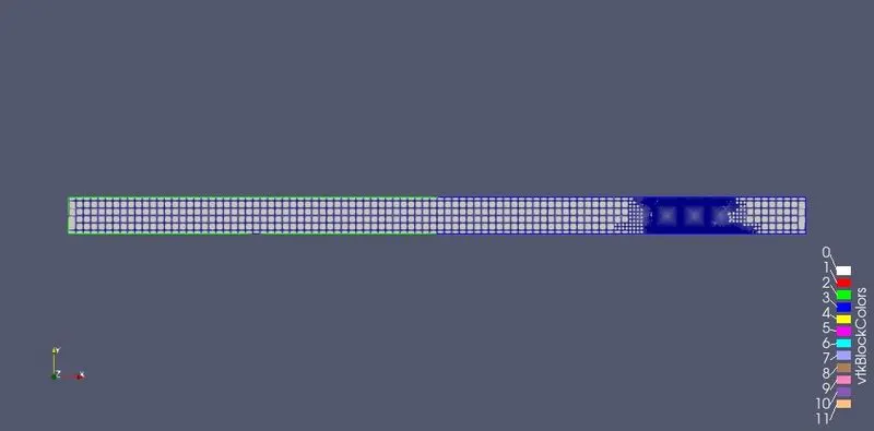
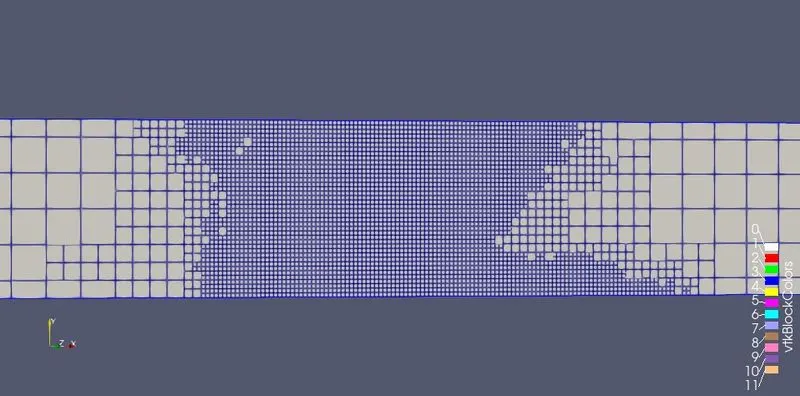
Mesh gets finer in certain region once the gases starts to mix during the simulation. The mesh gets refined by 3 stages with the smaller mesh size being 8 times lesser than the base mesh. The mesh gets refined in those regions where the concentration of N2 is within the given criterion value and this region keeps on changing during the simulation due to the movement of gases in the shocktube.
Animation:
The refined mesh keeps on varying in the region where there is contact between N2 and O2.
Mass Fraction N2:
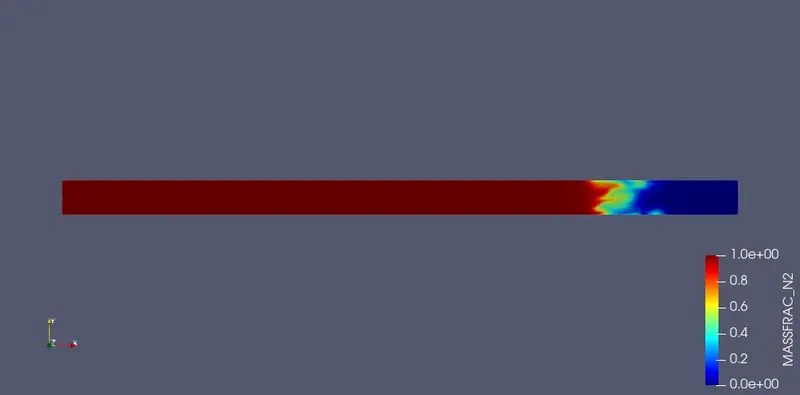
Since N2 is at high pressure, O2 cannot push N2. So O2 cannot enter the high pressure region and it is completely filled with N2.
Animation:
Mass Fraction O2:
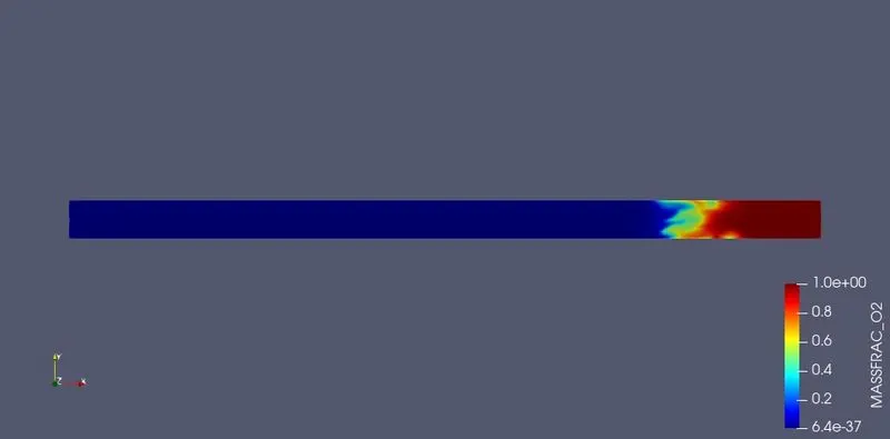
Since O2 is in low pressure region, O2 cannot push N2. So O2 cannot enter the high pressure region and it remains only at one end and resist mixing with N2 initially.
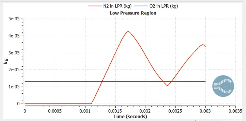
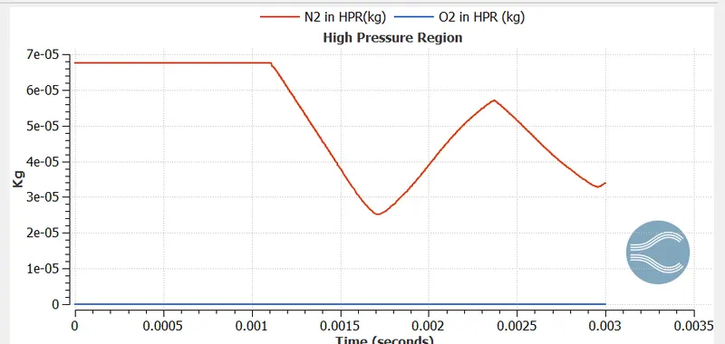
Since O2 will not be able to enter high pressure region, its concentration remains 0 and remains constant in Low pressure region. Mass of N2 decreases in high pressure region after diaphragm breaks and then keeps on fluctuating in both high pressure and low pressure regions since some portion of it enters low pressure region and its mass in high pressure region is being distributed with low pressure region.
Animation:
Pressure Contour:
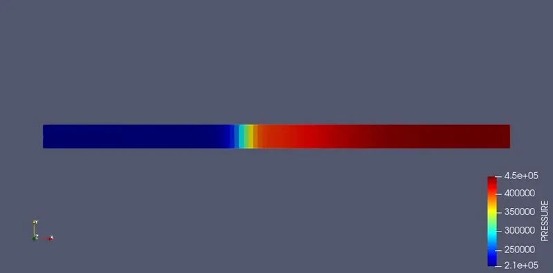
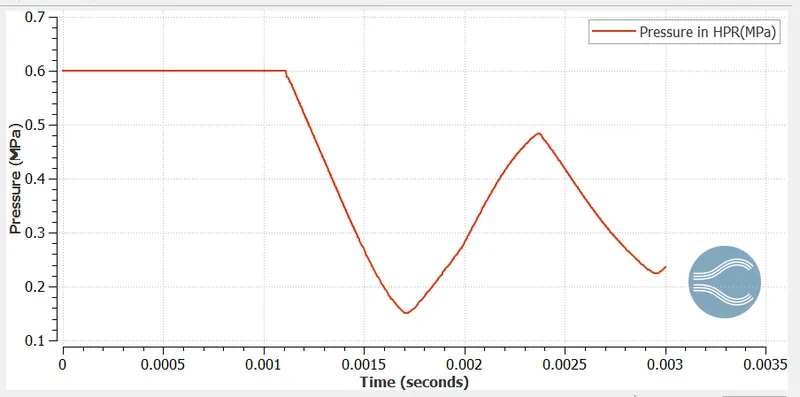
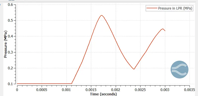
Gas in low pressure region, O2 is subjected to shock wave. After 0.001 sec which marks the breaking of diaphagrm, series of pressure waves are created compressing O2. This shock wave increases the pressure in low pressure region and pressure of 02. In simulation we can also see the waves getting reflected back moving N2 backward and forward, and this process continues till the intensity of shock waves reduces and dies down.
Animation:
Velocity Contour:
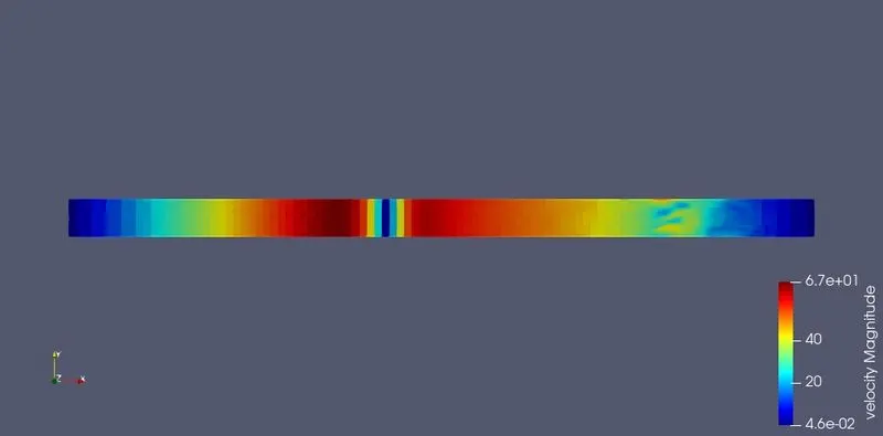
Since O2 resist the movement at the right side, velocity can be seen very low in that region. We can also see the O2 pushing N2 in the opposite direction and the velocity of the mixture continuosly varying throughout the simulation.
Animation:
Total Cell Count:
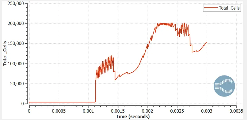
Once the gases starts to mix, due to the applied sub grid criterion for species in adaptive mesh refinement, the mesh gets refined in some regions where there is contact of N2 and O2. So due to the refined mesh, the number of cells in the domain increases after 0.001 sec. We can see the maximum of 200000 cells.
Temperature Contour:
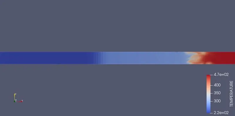
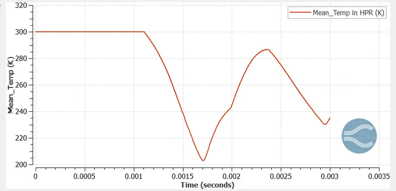
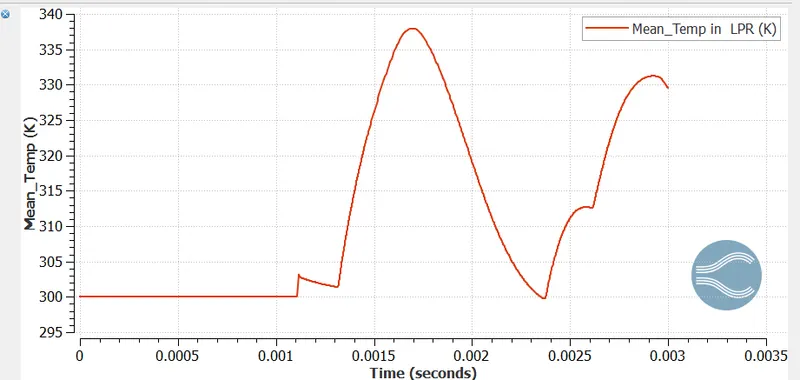
After 0.001 secs, Regions are made to open indicating the bursting of diaphragm. This leads to the expansion of high-pressure gas N2 and it produces a shock wave which passes through the low-pressure gas O2. The bursting diaphragm produces a series of pressure waves and they compress into a shock propagating through the driven gas O2. This shock wave increases the temperature in low pressure region and temperature of O2 and this goes on flcutuating in the simulation.
Animation:
Conclusion:
Succesfully simulated mixing of gases at higher and lower pressures and understood its chemical kinetics. Visualised the phenomenon of production of propogation of shock waves upon bursting of diaphagrm. Increase in temperature and pressure in low pressure region, production of reflecting shocks, motion of gases in shock ube upon mixing is also studied.
Understood the concept of Events in Convergeand its importance in simulating virtual bursting of diaphargm. Overview of adaptive mesh refinement in Converge is also studied and its importance in making mesh finer in certain regions to capture results accuractely is studied.