Week 7 - Simulation of a 1D Super-sonic nozzle flow simulation using Macormack Method

Aim:

• To simulate of the isentropic flow through a quasi 1D subsonic-supersonic nozzle using the McCormack’s technique in MATLAB.
• To derive both the conservation and non-conservation forms of the governing equations and solvee them using the MacCormack's technique
• To determine the steady-state distribution of the flow-field variables and investigate the difference between the two forms of governing equations by comparing their solutions.

Theory:

1D supersonic nozzle

Nozzle is made up of convergent and divergent section respectively and the location where the area is minimum is called the throat of the nozzle. The main advantage of this nozzle is that it increases the velocity of the flow. This type of nozzle is used in aircraft engines where there is a requirement to decrease the pressure to outer atmospheric pressure and increase the velocity of the exhaust to maximum level. In convergent section mach number is less than unity and is more than unity in divergent section and equal to unity at throat. All other variable like pressure, temperature and density of the fluid reduces as it passes through the nozzle.

Now we assume that Inlet (Subsonic section) is connected to the reservoir and inlet pressure, temperature, density are p0, t0, ρo.

At throat mach number which is the ratio of velocity of fluid to the local speed of sound is 1. Flow is expanded to supersonic speed(mach number greater than 1) in the divergent section and the variables are pe, te, ρe at the exit of the supersonic nozzle.The flow properties are assumed to be changing only along x-axis(only in 1-D). So it is said to be quasi-1D-flow. Area of the nozzle first decreases, reaches minimum at the throat and then increases. So the area of the nozzle changes as the function of distance taken along x-axis.

Governing equations

The governing equations describe how the values of the unknown variables (i.e. the dependent variables) change when one or more of the known (i.e. independent) variables change.

There are two forms of governing equations.

Conservative and Non conservative forms and these two forms in turn can be expressed in Integral form or in partial differential equation(PDE) form.

In conservative form the control volume will be stationary whereas in non-conservative form the control volume will be moving.

Governing equations for our problem

In Non-conservative form

Continuity Equation `(drho')/(dt') = (-rho'*(dv')/(dx'))-(rho'*v'*(d(lnA'))/(dx'))-(v'*(drho')/(dx'))`

Momentum Equation `(dv')/(dt') = (-v'*(dv')/(dx'))-(1)/gamma((dT')/(dx')+(T')/(p')*(dp')/(dx'))`

Energy Equation `(dT')/(dt') = (-v'*(dT')/(dx'))-(gamma-1)*T'*((dv')/(dx')+v'*(d(lnA'))/(dx'))`

These equations are non dimensionalised.

The non dimensionalised variables are

x’ = x/L L is the length of the nozzle

v’ = v/a₀ a₀ is the speed of sound

t’ = t/(L/ a₀)

A’ = A/A₀ where A₀ is the area of nozzle throat.

These equations are now solved using McCormack method.

The MacCormack method is a widely used discretization scheme for the numerical solution of partial differencial equations mostly for hyperbolic type. This second-order finite difference method and is explicit and is used in time marching solution. The technique consists to predictor method and corrector method and the average value of these two steps is used to update the solution for next time step and the time marching continues.

Predictor step

Here we make use of forward differencing for space derivatives in all governing equations which are first order. Variables ρ, v, t are updated and used in corrector step.

Corrector Step

Here we make use of backward differencing for space derivatives in all governing equations.

Average time step

Values from predictor and corrector steps are averaged out and are multiplied with dt and added with the older time step values thereby updating the solution.

Requirements to solve the Equation:

Mesh – the whole length of the nozzle is divided into certain number of equally spaced smaller lengths using grid points to create the mesh.

Discretization – For discretising the governing equations, we make use of the Mccormack technique with the above mentioned step.

Area of the nozzle,A first decreases, reaches minimum at the throat and then increases. So the area of the nozzle changes as the function of distance taken along x-axis. So area A is

A = 1 + (2.2*(x-1.5)²)

Initial conditions:

At time step t=0, values along the nozzle are

Density, ρ = 1 – 0.3146*x

Tempearture t = 1 – 0.2314*x

Velocity v=(0.1+1.09*x)*(`sqrt(t)`)

Boundary Conditions

Inlet Boundary conditions are

v(1) = 2*v(2) – v(3)

v(1) which is the velocity at node 1 is extrapolated using the values at node 2 and 3

Outlet boundary conditions are

v(n) = 2*v(n-1) – v(n-2)

ρ(n) = 2*ρ(n-1) – ρ(n-2)

t(n) = 2*t(n-1) – t(n-2)

here also the values at node n are extrapolated using 2 nodes before it.

Calculation of time step dt

dt = c (dx /(a+v))

c- CFL number for our problem it is taken as 0.5 – This gives the stable answer and CFL is the factor that determines the stability of the solution

a – local speed of sound a =(`sqrt(t)`) and v is the local velocity

the minimum value of this array is taken as the time step for our problem

This Time marching procedure(TMP) is carried out for 1400 iterations.

The final solutions pressure and Mach number are calculated as

Pressure `p = rho*t`

Mach number `M = v/(sqrt(t)`

Mass flow rate m = ρ * a * v

Using all these things the function for non conservative form is created in MATLAB.

MATLAB function for non-conservative form

  function [rho_nc,v_nc,t_nc,p_nc,mfr_nc,M_nc, rho_exact_nc,t_exact_nc,p_exact_nc,M_exact_nc, rho_thrt_nc,t_thrt_nc,p_thrt_nc,M_thrt_nc,v_thrt_nc, rho_resi_nc,t_resi_nc,v_resi_nc] = non_conser(x,dx,n,nt);
    
    %Solving quasi 1-D Supersonic Nozzle flow Simulation
    %MacCormack Method - Non-Conservative Form
    %nc in the code is Non-Conservative form
  
     %Inputs
     
     %Number of grid points
     n = 31;
     %Length of C-D Nozzle
     L =3;
     x = linspace(0,L,n);
     dx = x(2)-x(1);
     
     %Calculating Initial Profiles
     rho_nc = 1 - (0.3146 .* x);
     t_nc = 1 - (0.2314 .* x);
     v_nc = (0.1 + 1.09* x).*(t_nc.^0.5);
     
     %Area along Nozzle
     a = 1 + (2.2 .*(x - 1.5).^2);
     
     gamma = 1.4;
     
     %Time step 
     nt = 1400;
     %CFL Number
     c = 0.5;
     
     %step size dt
     dt = (c .*(dx./(v_nc +(t_nc.^0.5))));
     dt = min(dt);
     
     %Throat Index
     thrt_nc = find(a==1);
     
     %Outer Time loop
     for k = 1:nt
     
     %Keeping copy of precious time step value
     rho_old_nc = rho_nc;
     v_old_nc = v_nc;
     t_old_nc = t_nc;
     
         %Predictor Step   -------- Forward Differencing
         %Breaking down to various terms
         
         for j = 2:n-1
            dvdx = (v_nc(j+1) - v_nc(j))/dx;
            drhodx = (rho_nc(j+1) - rho_nc(j))/dx;
            dtdx = (t_nc(j+1) - t_nc(j))/dx;
            dlogadx = (log(a(j+1)) - log(a(j)))/dx;
            
            %Continuity Equation
            drhodt_p(j) = -(rho_nc(j).*dvdx) - (rho_nc(j).*v_nc(j).*dlogadx) - (v_nc(j).*drhodx);
            
            %Momentum Equation
            dvdt_p(j) = -(v_nc(j).*dvdx) - ((1/gamma)*(dtdx+((t_nc(j)./rho_nc(j)).*drhodx)));
            
            %Energy Equation
            dtdt_p(j) = -(v_nc(j).*dtdx) - (((gamma-1).*t_nc(j))*(dvdx + (v_nc(j).*dlogadx)));
            
            %Solution update
            rho_nc(j) = rho_nc(j) + (drhodt_p(j) * dt);
            v_nc(j) = v_nc(j) + (dvdt_p(j) * dt);
            t_nc(j) = t_nc(j) + (dtdt_p(j) * dt);
            
          end
          
          %Corrector Step    -------- Backward Differencing
          for j = 2:n-1
            dvdx = (v_nc(j) - v_nc(j-1))/dx;
            drhodx = (rho_nc(j) - rho_nc(j-1))/dx;
            dtdx = (t_nc(j) - t_nc(j-1))/dx;
            dlogadx = (log(a(j)) - log(a(j-1)))/dx;
            
            %Continuity Equation
            drhodt_c(j) = -(rho_nc(j).*dvdx) - (rho_nc(j).*v_nc(j).*dlogadx) - (v_nc(j).*drhodx);
            
            %Momentum Equation
            dvdt_c(j) = -(v_nc(j).*dvdx) - ((1/gamma)*(dtdx+((t_nc(j)./rho_nc(j)).*drhodx)));
            
            %Energy Equation
            dtdt_c(j) = -(v_nc(j).*dtdx) - (((gamma-1).*t_nc(j))*(dvdx + (v_nc(j).*dlogadx)));
            
          end
          
          %Computing Average Time Derivative
          drhodt = 0.5 * (drhodt_p + drhodt_c);
          dvdt = 0.5 * (dvdt_p + dvdt_c);
          dtdt = 0.5 * (dtdt_p + dtdt_c);
          
         
         %Final Solution Update
          
          for i = 2:n-1
              rho_nc(i) = rho_old_nc(i) + (drhodt(i)*dt);
              v_nc(i) = v_old_nc(i) + (dvdt(i)*dt);
              t_nc(i) = t_old_nc(i) + (dtdt(i)*dt);
          end
          
          %Boundary Conditions
          
          %Inlet BC
          v_nc(1) = 2 * v_nc(2) - v_nc(3);
          
          %Outlet BC
          v_nc(n) = 2*v_nc(n-1) - v_nc(n-2);
          rho_nc(n) = 2*rho_nc(n-1) - rho_nc(n-2);
          t_nc(n) = 2*t_nc(n-1) - t_nc(n-2);
          
          %Calculating Results
          
          %Mass Flow Rate
          mfr_nc = rho_nc .* a .* v_nc;
          
          %Mach Number
          M_nc = v_nc ./(t_nc.^0.5);
          
          %Pressure Ratio
          p_nc = rho_nc .* t_nc;
          
          %Calculating paramteres at throat at each iterations
          rho_thrt_nc(k) = rho_nc(thrt_nc);
          p_thrt_nc(k) = p_nc(thrt_nc);
          v_thrt_nc(k) = v_nc(thrt_nc);
          t_thrt_nc(k) = t_nc(thrt_nc);
          M_thrt_nc(k) = M_nc(thrt_nc);
          
          % Exact Analytical Solution at Throat after Steady State is reached
          rho_exact_nc = 0.634*ones(1,nt);
          t_exact_nc = 0.833*ones(1,nt);
          p_exact_nc = 0.528*ones(1,nt);
          M_exact_nc = 1*ones(1,nt);
          
          %Residual values at Throat Section (From Avearage of Predictor and Corrector)
          rho_resi_nc(k) = drhodt(thrt_nc);
          v_resi_nc(k) = dvdt(thrt_nc);
          t_resi_nc(k) = dtdt(thrt_nc);
          
          
##          %Plotting Mass flow rate at Different time steps
          figure(1)
          hold on
          if k==1
              plot(x,mfr_nc,'b')
              hold on
              grid on
          elseif k==50
              plot(x,mfr_nc,'k')
              hold on
          elseif k==100
              plot(x,mfr_nc,'m')
              hold on
          elseif k==300
              plot(x,mfr_nc,'-')
              hold on
          elseif k==700
              plot(x,mfr_nc,'r')
              hold on
          elseif k==1400
              plot(x,mfr_nc,'*')  
              grid on
              xlabel('Nozzle')
              ylabel('Mass Flow Rate')
              title('Mass flow rate at Different Time Steps --Non Conservative,n=31')
              legend('1dt','50dt','100dt','300dt','700dt','1400dt')
          end
        
        end
        
        %Plotting Figures
        
        %Non Conservative form -  Variation of Mach Number,Density,Pressure and Temperature at Throat with Time
        %Comparision of Exact analytical Values and Values from Code at Throat at each Time step
        figure(2)
        
        plot(M_thrt_nc,'k')
        hold on 
        plot(M_exact_nc,'r')
        xlabel('Time step')
        ylabel('Mach Number')
        legend('Varying with Time','Exact Value')
        title('Comparision of Exact and Time Varying Mach Number at Throat--Non Conservative')
        grid on
        
        figure(3)
        plot(rho_thrt_nc,'k')
        hold on 
        plot(rho_exact_nc,'r')
        xlabel('Time step')
        ylabel('Density')
        legend('Varying with Time','Exact Value')
        title('Comparision of Exact and Time Varying Density at Throat--Non Conservative')
        grid on
        
        figure(4)
        plot(p_thrt_nc,'k')
        hold on 
        plot(p_exact_nc,'r')
        xlabel('Time step')
        ylabel('Pressure')
        legend('Varying with Time','Exact Value')
        title('Comparision of Exact and Time Varying Pressure at Throat--Non Conservative')
        grid on
        
        figure(5)
        plot(t_thrt_nc,'k')
        hold on 
        plot(t_exact_nc,'r')
        xlabel('Time step')
        ylabel('Temperature')
        legend('Varying with Time','Exact Value')
        title('Comparision of Exact and Time Varying Temperature at Throat--Non Conservative')
        grid on
        
        
        % Mach number,Pressure,temperature,Density along nozzle after steady state is reached
        figure(6)
        
        subplot(4,1,1)
        plot(x,M_nc)
        hold on
        xlabel('Nozzle Length')
        ylabel('Mach Number')
        grid on
        title('Mach number,Pressure,Temperature,Density along Nozzle after Steady state is reached--Non Conservative')
        
        subplot(4,1,2)
        plot(x,t_nc)
        xlabel('Nozzle Length')
        ylabel('Temperature')
        grid on
        
        subplot(4,1,3)
        plot(x,rho_nc)
        xlabel('Nozzle Length')
        ylabel('Density')
        grid on
        
        subplot(4,1,4)
        plot(x,p_nc)
        xlabel('Nozzle Length')
        ylabel('Pressure')
        grid on
        
       %Residual Plot -----These are the values multiplied with dt and are added to older values. These are the ones that update the solution
      %if these are equal to zero, it means solution is no longer getting updated and solution has become stable

        figure(7)
        
        plot(rho_resi_nc,'k')
        hold on
        plot(v_resi_nc,'b')
        plot(t_resi_nc,'r')
        xlabel('Time step')
        ylabel('Residual Values')
        title('Non Conservative Form- Residuals,n=31')
        legend('Density','Velocity','Temperature')
        grid on
        
        
        
        
        
      end
      
          
          
         
           
         

Explanation of Code:

Function with all the required outputs is defined for non conservative form. The outputs include all primitive variables like density, velocity, temperature, pressure, mass flow rate and mach number along the nozzle. Exact analytical values of these variables at throat, Variables calculated from MacCormack method at the throat of nozzle, and the residual values of the variables.

Initially the number of grid points is defined in n and the length of the nozzle is equally divided to n points creating the mesh of the domain.

Minimum value of dt is taken as time step and dt is calculated using CFL =0.5 as it will produce the stable result. Area along the nozzle is defined and initial profile of variables is created using the formulae. Index of the throat section of the nozzle is determined as this will used to find out the values of variables at throat for all 1400 iterations.

Time marching procedure is carried out for 1400 iterations and for time=1400*dt. Outer time loop for 1400 time steps is initialized and the MacCormack method is coded inside the loop. Predictor uses forward differencing and variable profiles are updated in the step and these updated values are used in corrector step which is backward differencing. Average value of predictor and corrector is calculated.

For the final solution update, for loop is used and the old values are added with the product of corrector step and dt. Initial conditions and boundary conditions are provided and the required outputs- mass flow rate, mach number and pressure along the nozzle are calculated using density, temperature and velocity profiles obtained from the code.

Variables at the throat section are retrieved for all 1400 iterations and the exact analytical values at throat are created having sixe of 1*1400. These values will be used for comparision and to see the accuracy of the MacCormack method. Residual values are also taken and constant values of residuals indicate that the solution is no longer changing and it has reached steady state. The required graphs are plotted.

Conservative Form

In this form the control volume is stationary.

Governing equations in conservative form

Solution Vector

`u1 = rho *a`

`u2 = rho * a*v`

`u3 = ρ(t/(gamma-1)-(gamma/2)*v^2)`

Flux terms are

`f1 = rho*a*v`

`f2 = (rho*a*v^2 ) + ((1/gamma)*rho*a)`

`f3 = rho(e/(gamma-1)-gamma/2*v^2)*v*a +(rho*a*v)`

There is one source term

`j2 = 1/gamma*rho*(da)/dx`

Finally our equations can be written as

`(du1)/dt = -(df1)/dx`

`(du2)/dt = -(df2)/dx + j2`

`(du3)/dt = -(df3)/dx`

Primitive Variables:

Using the above equations and performing some mathematical manipulations we can get required updated primitive variables v, ρ, t, pressure and Mach number.

Density ρ = u1/a

Velocity v = u2/u1

Temperature `t = (gamma-1)*((u3)/(u1)- gamma/2*v^2)`

Pressure p = ρ*t

Mach number M = (v/t^1/2)

Mass flow rate m = ρ * a * v

The MacCormack method is carried out just like non conservative form. But the solution vector, flux terms and all the primitive variables are need to be updated at each step. Calculation of dt is same as the non conservative form and is carried out for 1400 iterations using time marching procedure.

Initial conditions

For 0<=x<0.5

ρ = 1 ;

t = 1 ;

for 0.5<=x<=1.5

ρ= 1 - (0.3146 * (x-0.5));

t = 1 - (0.167* (x-0.5));

for 1.5<=x<=3.5

ρ = 0.634 - (0.3879 * (x-1.5));

t= 0.833 - (0.3507 * (x-1.5));

velocity, v = u2

pressure p = ρ*t

mach number M =(v/t^1/2)

Boundary conditions

Inlet Boundary conditions

u1(1) = ρ*a

u2(1) = 2*u2(2) – u2(3)

u3(1) = 2*u3(2) – u3(3)

MATLAB function for Conservative form

  function [rho_c,v_c,t_c,p_c,mfr_c,M_c, rho_exact_c,t_exact_c,p_exact_c,M_exact_c, rho_thrt_c,t_thrt_c,p_thrt_c,M_thrt_c,v_thrt_c, rho_resi_c,t_resi_c,v_resi_c] = conser(x,dx,n,nt,gamma);
    
    %Solving quasi 1-D Supersonic Nozzle flow Simulation
    %MacCormack Method - Conservative Form
    %c in the function for most variables means conservative form
    
    
     %Inputs
     
     %Number of grid points
     n = 31;
     %Length of C-D Nozzle
     L =3;
     x = linspace(0,L,n);
     dx = x(2)-x(1);
     
     %Area along Nozzle
     a = 1 + (2.2 .*(x - 1.5).^2);
     
     
     %Calculating Initial Profiles
     for i=1:n
         if(x(i)>=0 && x(i)<=0.5)
             rho_c(i) = 1 ;
             t_c(i) = 1 ;
          elseif(x(i)>0.5 && x(i)<=1.5)
             rho_c(i) = 1 - (0.3146 * (x(i)-0.5));
             t_c(i) = 1 - (0.167* (x(i)-0.5));
          else
             rho_c(i) = 0.634 - (0.3879 * (x(i)-1.5));
             t_c(i) = 0.833 - (0.3507 * (x(i)-1.5));
           end
      end
      
      %Calculating Initial Velcoity and Pressure profile
      v_c = 0.59./(rho_c.*a);
      p_c =rho_c.*v_c;
     
     gamma = 1.4;
     
     %Time step 
     nt = 1400;
     %CFL Number
     c = 0.5;
     
     %step size dt
     dt = (c .*(dx./(v_c +(t_c.^0.5))));
     dt = min(dt);
     
     %Throat Index
     thrt_c = find(a==1);
     
     
     %Initialising Solution Vector
     u1 = rho_c.*a;
     u2 = rho_c.*a.*v_c;      %u1.*v_c
     u3 = u1.*((t_c./(gamma-1)) + ((gamma/2).*(v_c.^2)));
     
     
     %Outer Time loop
     for k = 1:nt
     
     %Keeping copy of precious time step value
     u1_old = u1;
     u2_old = u2;
     u3_old = u3;
     
     %Initial Flux Terms
     f1 = u2;
     f2 = ((u2.^2) ./u1) + (((gamma-1)/gamma) .* (u3 -((gamma/2).*((u2.^2)./u1))));
     f3 = ((gamma.*u2.*u3)./u1) - ((gamma.*(gamma-1).*(u2.^3))./(2.*(u1.^2)));
 
         %Predictor Step   -------- Forward Differencing
         %Breaking down to various terms
         
         for j = 2:n-1
            
            df1dx(j) = (f1(j+1) - f1(j))/dx;
            df2dx(j) = (f2(j+1) - f2(j))/dx;
            df3dx(j) = (f3(j+1) - f3(j))/dx;
            
            %Source Term J2
            dadx(j) = (a(j+1) - a(j))/dx;
            j2_p(j) = ((1/gamma)*((rho_c(j)*t_c(j))*dadx(j)));
            
            %Continuity Equation
            du1dt_p(j) = -(df1dx(j));
            
            %Momentum Equation
            du2dt_p(j) = (-df2dx(j) + j2_p(j));
            
            %Energy Equation
            du3dt_p(j) = -(df3dx(j));
            
            %Solution update
            u1(j) = u1(j) + (du1dt_p(j) * dt);
            u2(j) = u2(j) + (du2dt_p(j) * dt);
            u3(j) = u3(j) + (du3dt_p(j) * dt);
            
          end
          
          %Retriving updated Primitive Variables Density,Temperature,Velocity from updated Solution Vector u1,u2,u3
          %Mathematical Modulation of u1,u2 and u3 equations.
          rho_c = u1./a;
          v_c = u2./u1;
          t_c = (gamma-1).*((u3./u1)-((gamma/2).*(v_c.^2)));
          
          %Updating Flux Terms before Corrector step
          f1 = u2;
          f2 = ((u2.^2) ./u1) + (((gamma-1)/gamma) .* (u3 -((gamma/2).*((u2.^2)./u1))));
          f3 = ((gamma.*u2.*u3)./u1) - ((gamma.*(gamma-1).*(u2.^3))./(2.*(u1.^2)));
          
          
          %Corrector Step    -------- Backward Differencing
          for j = 2:n-1
            
            df1dx(j) = (f1(j) - f1(j-1))/dx;
            df2dx(j) = (f2(j) - f2(j-1))/dx;
            df3dx(j) = (f3(j) - f3(j-1))/dx;
            
            %Source Term J2
            dadx(j) = (a(j) - a(j-1))/dx;
            j2_c(j) = ((1/gamma)*((rho_c(j)*t_c(j))*dadx(j)));
            
            %Continuity Equation
            du1dt_c(j) = -(df1dx(j));
            
            %Momentum Equation
            du2dt_c(j) = (-df2dx(j) + j2_c(j));
            
            %Energy Equation
            du3dt_c(j) = -(df3dx(j));
            
          end
          
          
          %Computing Average Time Derivative
          du1dt = 0.5 * (du1dt_p + du1dt_c);
          du2dt = 0.5 * (du2dt_p + du2dt_c);
          du3dt = 0.5 * (du3dt_p + du3dt_c);
          
         
         %Final Solution Update
          
          for i = 2:n-1
              u1(i) = u1_old(i) + (du1dt(i)*dt);
              u2(i) = u2_old(i) + (du2dt(i)*dt);
              u3(i) = u3_old(i) + (du3dt(i)*dt);
          end
          
          %Boundary Conditions
          
          %Inlet BC
          u1(1) = rho_c(1)*a(1);
          u2(1) = 2 * u2(2) - u2(3);
          
          %velocity at first node
          v_c(1) = u2(1)/u1(1);
          u3(1) = u1(1)*((t_c(1)/(gamma-1)) + ((gamma/2).*(v_c(1)^2)));
         
          %Outlet BC
          u1(n) = 2*u1(n-1) - u1(n-2);
          u2(n) = 2*u2(n-1) - u2(n-2);
          u3(n) = 2*u3(n-1) - u3(n-2);
          
          %Updating Prmitive Variables Density,Temperature,Velocity from updated Solution Vector u1,u2,u3
          %Again the Mathematical Modulation of u1,u2 and u3 equations.
          rho_c = u1./a;
          v_c = u2./u1;
          t_c = (gamma-1).*((u3./u1)-((gamma/2).*(v_c.^2)));
          
          
          
          %Calculating Results
          
          %Mass Flow Rate
          mfr_c = rho_c .* a .* v_c;
          
          %Mach Number
          M_c = v_c ./(t_c.^0.5);
          
          %Pressure Ratio
          p_c = rho_c .* t_c;
          
          %Calculating paramteres at throat at each iterations
          rho_thrt_c(k) = rho_c(thrt_c);
          p_thrt_c(k) = p_c(thrt_c);
          v_thrt_c(k) = v_c(thrt_c);
          t_thrt_c(k) = t_c(thrt_c);
          M_thrt_c(k) = M_c(thrt_c);
          
          % Exact Analytical Solution at Throat after Steady State is reached
          rho_exact_c = 0.634*ones(1,nt);
          t_exact_c = 0.833*ones(1,nt);
          p_exact_c = 0.528*ones(1,nt);
          M_exact_c = 1*ones(1,nt);
          
          %Residual values at Throat Section (From Avearage of Predictor and Corrector)
          rho_resi_c(k) = du1dt(thrt_c);
          v_resi_c(k) = du2dt(thrt_c);
          t_resi_c(k) = du3dt(thrt_c);
          
          
##          %Plotting Mass flow rate at Different time steps
          figure(8)
          hold on
          if k==1
              plot(x,mfr_c,'b')
              hold on
              grid on
          elseif k==50
              plot(x,mfr_c,'k')
              hold on
          elseif k==100
              plot(x,mfr_c,'m')
              hold on
          elseif k==300
              plot(x,mfr_c,'-')
              hold on
          elseif k==700
              plot(x,mfr_c,'r')
              hold on
          elseif k==1400
              plot(x,mfr_c,'*')  
              grid on
              xlabel('Nozzle')
              ylabel('Mass Flow Rate')
              title('Mass flow rate at Different Time Steps--Conservative Form,n=31')
              legend('1dt','50dt','100dt','300dt','700dt','1400dt')
          end
        
        end
        
        %Plotting Figures
        
        %Conservative form -  Variation of Mach Number,Density,Pressure and Temperature at Throat with Time
        %Comparision of Exact analytical Values and Values from Code at Throat at each Time step
        figure(9)
        
        plot(M_thrt_c,'k')
        hold on 
        plot(M_exact_c,'r')
        xlabel('Time step')
        ylabel('Mach Number')
        legend('Varying with Time','Exact Value')
        title('Comparision of Exact and Time Varying Mach Number at Throat--Conservative Form')
        grid on
        
        figure(10)
        plot(rho_thrt_c,'k')
        hold on 
        plot(rho_exact_c,'r')
        xlabel('Time step')
        ylabel('Density')
        legend('Varying with Time','Exact Value')
        title('Comparision of Exact and Time Varying Density at Throat--Conservative Form')
        grid on
        
        figure(11)
        plot(p_thrt_c,'k')
        hold on 
        plot(p_exact_c,'r')
        xlabel('Time step')
        ylabel('Pressure')
        legend('Varying with Time','Exact Value')
        title('Comparision of Exact and Time Varying Pressure at Throat--Conservative Form')
        grid on
        
        figure(12)
        plot(t_thrt_c,'k')
        hold on 
        plot(t_exact_c,'r')
        xlabel('Time step')
        ylabel('Temperature')
        legend('Varying with Time','Exact Value')
        title('Comparision of Exact and Time Varying Temperature at Throat--Conservative Form')
        grid on
        
        
        % Mach number,Pressure,temperature,Density along nozzle after steady state is reached
        figure(13)
        
        subplot(4,1,1)
        plot(x,M_c)
        hold on
        xlabel('Nozzle Length')
        ylabel('Mach Number')
        grid on
        title('Mach number,Pressure,Temperature,Density along Nozzle after Steady state is reached--Conservative Form')
        
        subplot(4,1,2)
        plot(x,t_c)
        xlabel('Nozzle Length')
        ylabel('Temperature')
        grid on
        
        subplot(4,1,3)
        plot(x,rho_c)
        xlabel('Nozzle Length')
        ylabel('Density')
        grid on
        
        subplot(4,1,4)
        plot(x,p_c)
        xlabel('Nozzle Length')
        ylabel('Pressure')
        grid on
        
        %Residual Plot -----These are the values multiplied with dt and are added to older values. These are the ones that update the solution
        %if these are equal to zero, it means solution is no longer getting updated and solution has become stable
        figure(14)
        
        plot(rho_resi_c,'k')
        hold on
        plot(v_resi_c,'b')
        plot(t_resi_c,'r')
        xlabel('Time step')
        ylabel('Residual Values')
        title('Conservative Form- Residuals,n=31')
        legend('Density','Velocity','Temperature')
        grid on
        
        
        
        
        
      end
      
          
          
         
           
         

Main Code

MATLAB code to call both functions and to plot graphs to compare both forms

           clear all
           close all
           clc
           
           %Simulation of 1--D Supersonic Nozzle Flow
           %MacCormack Method
           %Comparative Study of Conservative and Non Conservative Form
           %Using function of both Conservative and Non Conservative form to plot graphs
           
           
           
           %Number of grid points
           n = 31;
           %Length of C-D Nozzle
           L =3;
           x = linspace(0,L,n);
           dx = x(2)-x(1);
           nt = 1400;
           gamma = 1.4;
           
           %Calling Non-Conservative form function
           [rho_nc,v_nc,t_nc,p_nc,mfr_nc,M_nc, rho_exact_nc,t_exact_nc,p_exact_nc,M_exact_nc, rho_thrt_nc,t_thrt_nc,p_thrt_nc,M_thrt_nc,v_thrt_nc, rho_resi_nc,t_resi_nc,v_resi_nc] = non_conser(x,dx,n,nt);
  
           %Calling Non-Conservative form function
           [rho_c,v_c,t_c,p_c,mfr_c,M_c, rho_exact_c,t_exact_c,p_exact_c,M_exact_c, rho_thrt_c,t_thrt_c,p_thrt_c,M_thrt_c,v_thrt_c, rho_resi_c,t_resi_c,v_resi_c] = conser(x,dx,n,nt,gamma);
            
           
           %Plotting Comparative Graphs of both forms
       
           % Mach number,Pressure,temperature,Density along nozzle after steady state is reached
           
          figure(15)
          plot(x,M_nc)
          hold on
          plot(x,M_c,'*')
          xlabel('Nozzle Length')
          ylabel('Mach Number')
          legend('Non Conservative','Conservative')
          grid on
          title('Comparision of Mach number along Nozzle length after Steady state is reached')
          
          figure(16)
          plot(x,rho_nc)
          hold on
          plot(x,rho_c,'*')
          xlabel('Nozzle Length')
          ylabel('Density')
          legend('Non Conservative','Conservative')
          grid on
          title('Comparision of Density along Nozzle length after Steady state is reached')
          
          figure(17)
          plot(x,p_nc)
          hold on
          plot(x,p_c,'*')
          xlabel('Nozzle Length')
          ylabel('Pressure')
          legend('Non Conservative','Conservative')
          grid on
          title('Comparision of Pressure along Nozzle length after Steady state is reached')
          
          figure(18)
          plot(x,t_nc)
          hold on
          plot(x,t_c,'*')
          xlabel('Nozzle Length')
          ylabel('Temperature')
          legend('Non Conservative','Conservative')
          grid on
          title('Comparision of Temperature along Nozzle length after Steady state is reached')
          
          
          %Comparing Mass Flow Rate along Nozzle after Steady State is Reached
          
          figure(19)
          plot(x,mfr_nc,'k')
          hold on
          plot(x,mfr_c,'r')
          xlabel('Nozzle Length')
          ylabel('Mass Flow Rate')
          legend('Non Conservative','Conservative')
          grid on
          title('Comparision of Mass Flow Rate along Nozzle length after Steady state is reached,n=31')

Code in the function of conservative part is almost similar to non conservative part and in the main function both functions are called and the required graphs are plotted for comparing both the methods.

Result and Conclusions:

The following are the required results the need to be evaluated from MacCormack method

Steady-state distribution of primitive variables inside the nozzle
Time-wise variation of the primitive variables
Variation of Mass flow rate distribution inside the nozzle at different time steps during the time-marching process
Comparison of Normalized mass flow rate distributions of both forms

Outputs from the Non conservative form of MacCormack method.

Non-Conservative Form:

Variation of Non-Dimensional Mach Number,Pressure,Density and Temperature along the Nozzle

Steady-state Distribution of Primitive variables inside the Nozzle

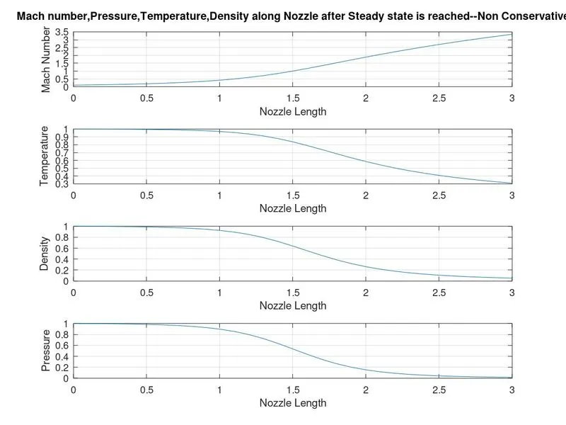
It can be seen from the plot that the mach number is increasing continuousy from the subsonic to supersonic(mach>1)to about 3.4 through the supersonic nozzle inlet to outlet. This is the exact output desired from the nozzle. And all other non dimensional variables are reducing through the nozzle. So the non-conservative form of MacCormack method can be relied to simulate the flow.

Comaprision of Exact Analytical Values of Variables and Time varying solution at Throat of Nozzle for 1400 time steps

How close the values of variables at Throat in comparison to the exact analytical values

Time-wise Variation of Primitive Variables at Throat

Comparing Non dimensional Mach Number

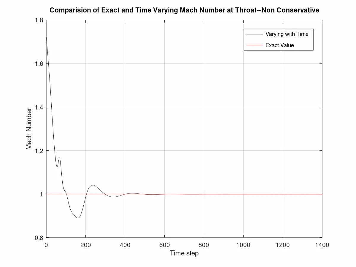
The mach number at nozzle is nore than 1 at initial iterations and decreases below 1, oscialltes above and below 1 for some iterations. After 500 -600 iteratons the mach number beconmes stable for the rest of the time steps and is also close to the exact analytical value. The stable solution after 600 iterations is 0.999 which is not a big difference. So the mach number at throat from non conservative form. The condition is true for other variables like pressure, temperature and denisty at throat.

Comparing Non dimensional Pressure

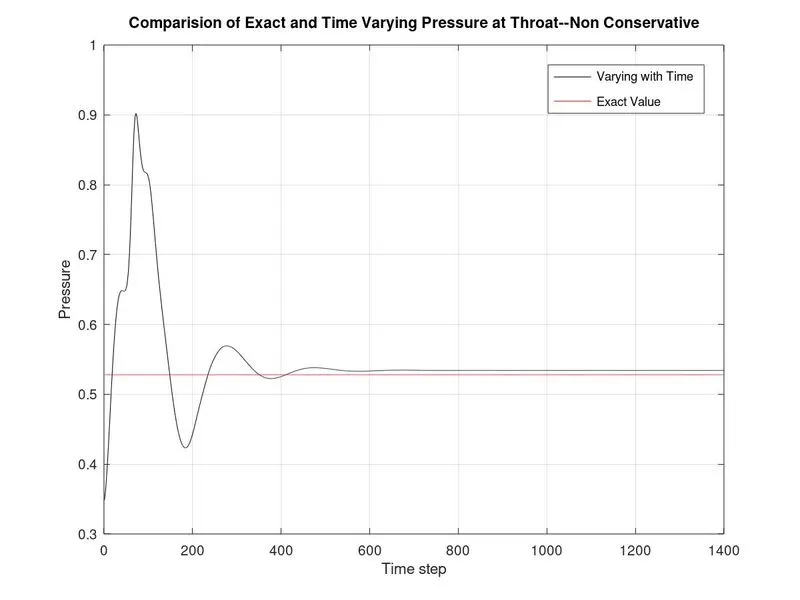
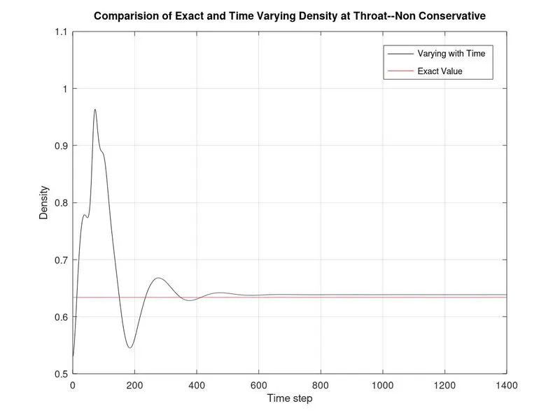
Pressure at throat oscillates above and below the exact solution for 600 iterations. Pressure becomes stable after 600 iterations and the difference between them is not much larger. Again the outputs are worth here in non consevative form. The same is true for density and temperature.

Comparing Non dimensional Density

Comparing Non dimensional Temperature

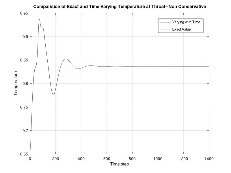
Temperature at throat as other variables oscillates around exact solution for 600 iterations and becomes stable after. The solution is little above exact solution and the difference is little bit.
All primitive variables in non conservative form brushes near exact solution after 600 iterations and this form is better one as solution compromises with exact solution.

Conservative Form:

Outputs from the Conservative form of MacCormack method.

Variation of Non-Dimensional Mach Number,Pressure,Density and Temperature along the Nozzle

Steady-state Distribution of Primitive variables inside the Nozzle

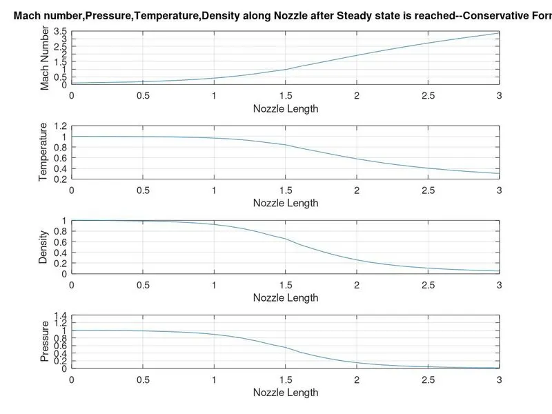
It can be seen from the plot that the mach number is increasing continuousy from the subsonic to supersonic(mach>1) through the supersonic nozzle inlet to outlet. This is the exact output desired from the nozzle. And all other non dimensional variables are reducing through the nozzle. So the conservative form of MacCormack method can be relied to simulate the flow but how close these values to eact solution need to be studied.

Comaprision of Exact Analytical Values of Variables and Time varying solution at Throat of Nozzle for 1400 time steps

How close the values of variables at Throat in comparison to the exact analytical values

How primitive variables are getting updated with time--Time Marching

Time-wise Variation of Primitive Variables at Throat

Comparing Non dimensional Mach Number

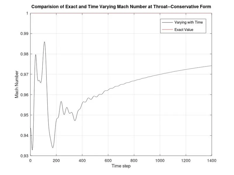
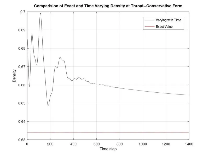
Exact mach number at throat is 1 and from the conservative form, the mach number is constantly changing and at start it is around 0.935 and it oscillates for 500 iterations between 0.935 and 0.985. After 500 iterations it increases continuously from 0.96. Althought the mach number really never reach the exact mach number 1 also its not steady. So there is much difference between analytical value and time varying value in comparision to Non conservative form. So these values are obtained better in non conservative form. There is huge margin between mach number and exact mach number here.
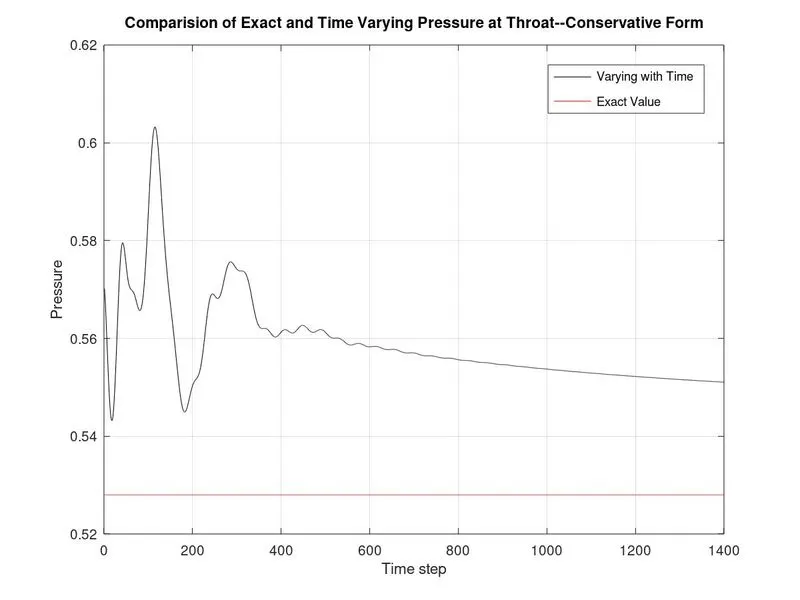
This is same for other primitive variables at throat in conservative form.

Comparing Non dimensional Pressure

Comparing Non dimensional Density

Comparing Non dimensional Temperature

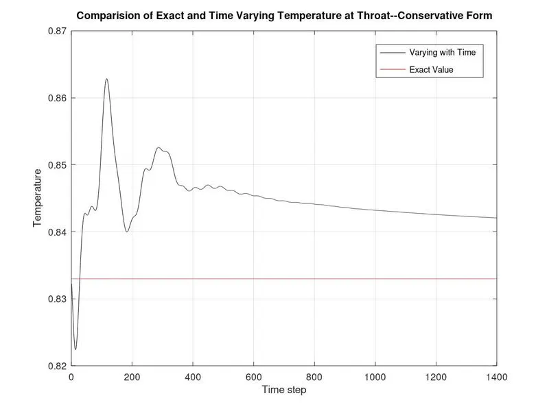
All primitive variables in conservative form do not reach the exact analytical value through out 1400 iterations and there is much difference between them in compared to non conservative form. So non conservative form produces values near to exact values and stable values after 600-700 iterations. in conservative form, the solution keeps on oscillating and maintains more gap between exact value.

So non conservative form produces variables that are stable after 600 iterations and difference is not big as in conservative form, which makes the non conservative form better one for primitive variables at throat.

The condition may not be same for values at different position in the nozzle.

Grid Independent Study:

When any of the CFD problems are solved, solution should not be affected by the size of the grid. Grid independent study is carried out to ensure that our solution is independent on the grid size. So we will try to solve the problem with more number of nodes making the domain finer. Grid may be coarse, medium or finer. More the number of nodes, lesser the grid size and finer the mesh is. So the number of nodes is doubled in our study and the effect of this on the solution is evaluated.

Upon changing the number of nodes, if the difference between the solutions in not much larger, then the method can be said grid independent. Now let’s compare the values of the variables at throat after attaining the steady state for both conservative and non conservative form for nodes n=31 and n=61.

Non dimensional Primitive variables at Throat of nozzle after Steady state is reached.

Method/Form	Grid Points	Pressure	Temperature	Mach number
Exact Analytical Solution	-	0.528	0.833	1
Conservative	n=31	0.551	0.842	0.974
Non Conservative	n=31	0.534	0.836	0.999
Conservative	n=61	0.549	0.842	0.973
Non Conservative	n=61	0.532	0.835	0.999

It can be seen from above table that the non conservative form produces values that are nearly equal to the exact analytical values. Conservative form also produces values which do not have bigger differences like 0.5. Comparing both forms at nodes n=31 and n=61, non conservative form yields better and compromising values at nozzle throat.
When number of nodes is doubled, the solution produced do not vary in the same form. They almost match their respective forms. So we can say that our solution is not getting affected by the change in the number of nodes making solution grid independent.

Residual Values

These are the values which are multiplied to dt and added to the older values of primitive variables. These are the values which update the solution to the newer time step. If these values are near zero or zero means that our solution is no more getting or the solution has converged.

When the residuals become constant, then solution is obtained or said to be converged.

Non Conservative Form Residuals of variables for 1400 time steps:

for n=31

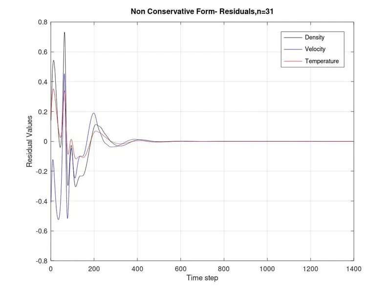
Residuals are ones that update the solution in each step in time marching procedure.
For around 500 iterations,residual values of variables oscillate between 0.7 and -0.5 indicating the solution getting updated till 500 iterations. Any constant value near 0 reflects that update in the solution is not much and this indicates solution is reaching steady state and this can be seen after 600 iterations where all residual values of variables are constant or approaching zero and not varying much.

for n=61

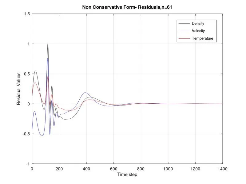
Here the values oscillate for around 900 iterations with increased amplitude on both sides. This can be inferred as increase in number of nodes increases the residual values and this increases the time to reach the convergence in solution although solutions aren't affected much. So increase in number of nodes doesnt affect the solution but increases the time to reach convergence of solution.

Conservative Form Residuals of variables for 1400 time steps:

for n=31

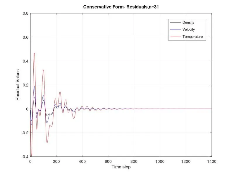
Compared to non conservative form when n=31, residual values keeps on changing for more number of time steps leading the convergence of solution with increased time. Here also the solution is not much affected as the final solution is stable and can be relied on but takes large number of time steps.

for n=61

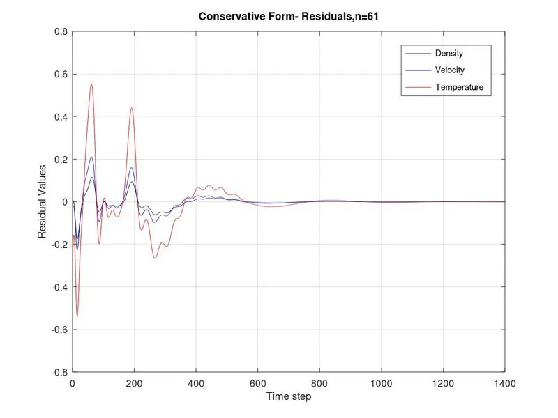
Here also compared to non conservative form when n=61, residual values keeps on changing for more number of time steps leading the convergence of solution with increased time. Here also the solution is not much affected as the final solution is stable and can be relied on but takes large number of time steps.

So it can be concluded that increasing the number of nodes increases the time to converge the solution in both conservative and non conservative form. For same number of nodes, solution becomes stable in non conservative form faster with less number of time steps than conservative form. Althought solution obtained in each case are good enough and stable.

Mass-Flow Rate:

The variation of Non Dimensional Mass Flow Rate at different time steps, mass flow along the nozzle after steady state is reached, for varying number of grid points obtained from both conservative and non conservative form.

Non Conservative Form

Mass flow rate along the nozzle at different time step

for f=31

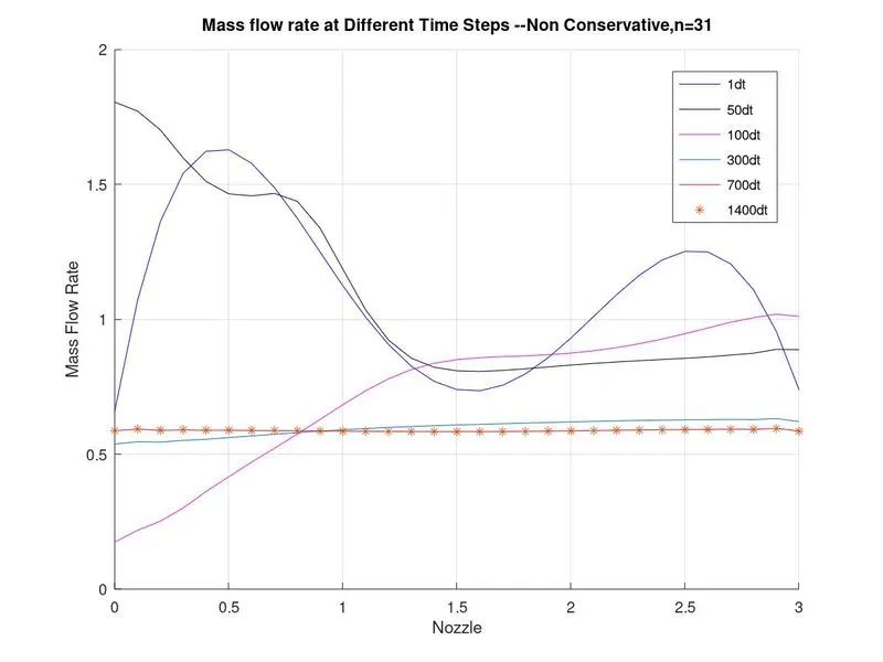
It can be seen that at initial time steps the mass flow rate across nozzle is not constant. For 700 and 1400th time steps, when the solution has become stable, mass flow rate is almost constant along nozzle length and around 0.58 to 0.6.

for n=61

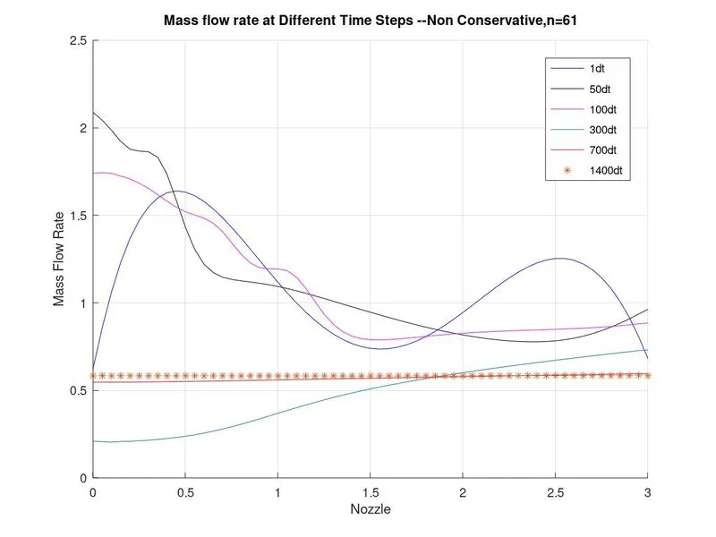
With increase in nodes, again it can be seen that at initial time steps the mass flow rate across nozzle is not constant keeps on varying. For 700 and 1400th time steps, mass flow rate is almost constant along nozzle length with value around 0.58 to 0.6.

Conservative Form

Mass flow rate along the nozzle at different time step

for n=31

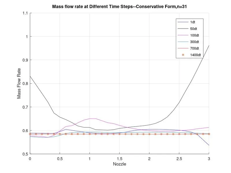
Mass flow rate varies much till 300 iterations and it becomes stable for lesser number of iterations compared to non conservative form. The reason is that the initial consitions in both cases aren't same and however this form produces stable mass flow rate within leseer time steps. Mass flow rate value vary with time steps after 300, but for the same time step values are constant along the nozzle.

for n=61

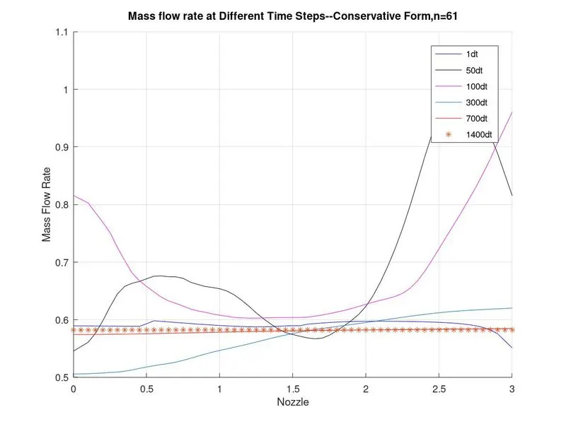
With increase in number of nodes, Mass flow rate takes larger time step to become constant along nozzle. Mass flow rate value vary with time steps after 700, but for the same time step values are constant along the nozzle after 700 time steps here.

The comparision between both the forms for equal number of nodes after solution converges needs to be evaluated.

Comparision of Conservative and Non Conservative Forms of MacCormack Method:

Comparision of non dimensional Mass Flow Rate along Nozzle length of Conservative and Non conservative Forms after Steady State is Reached

for n=31

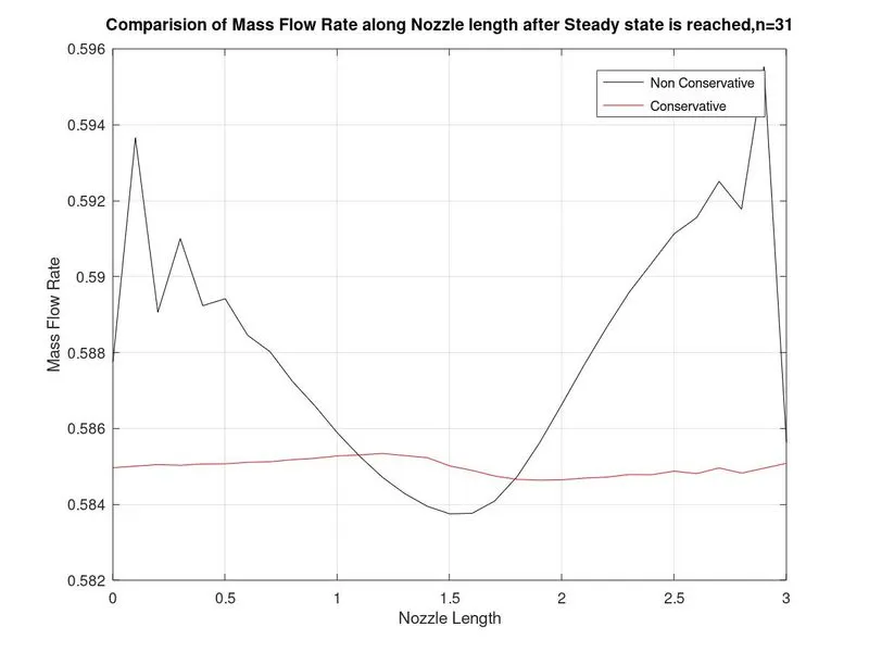
For n=31 in both forms, after solution getting stable, mass flow rate is more constant along the nozzle in conservative form. The values along the nozzle is between 0.584 and 0,586 at all nodes in conservative form where as values vary much in non conservative form. But the extent at which vary is not that big because they vary between 0.583 and 0.595 which does not make big difference but one has to accept that mass flow rate is much more constant along nozzle in conservative form.

for n=61

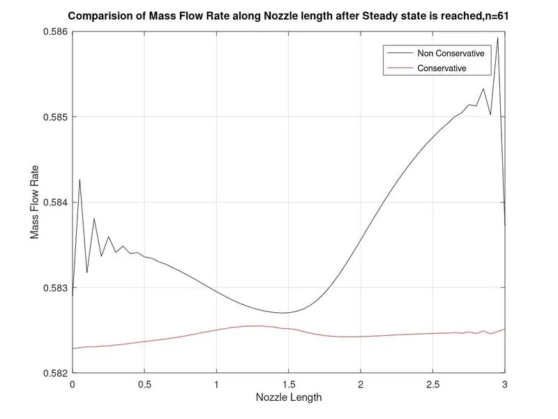
For n=61 in both forms, after solution getting stable, mass flow rate is more constant along the nozzle in conservative form. The values along the nozzle is between 0.584 and 0,583 at all nodes in conservative form but mass flow rate doesnt vary as much as when n=31 in non conservating form.

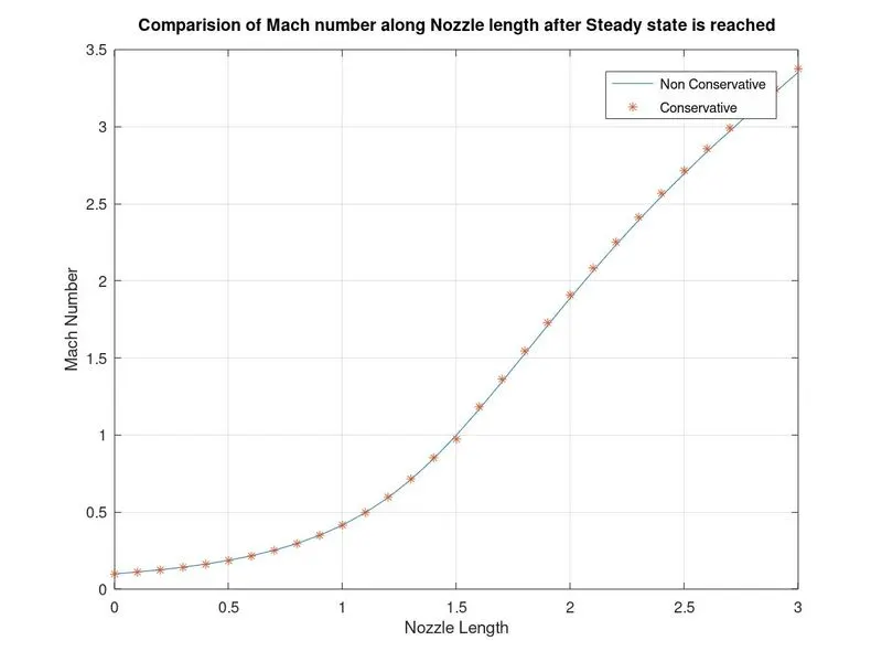
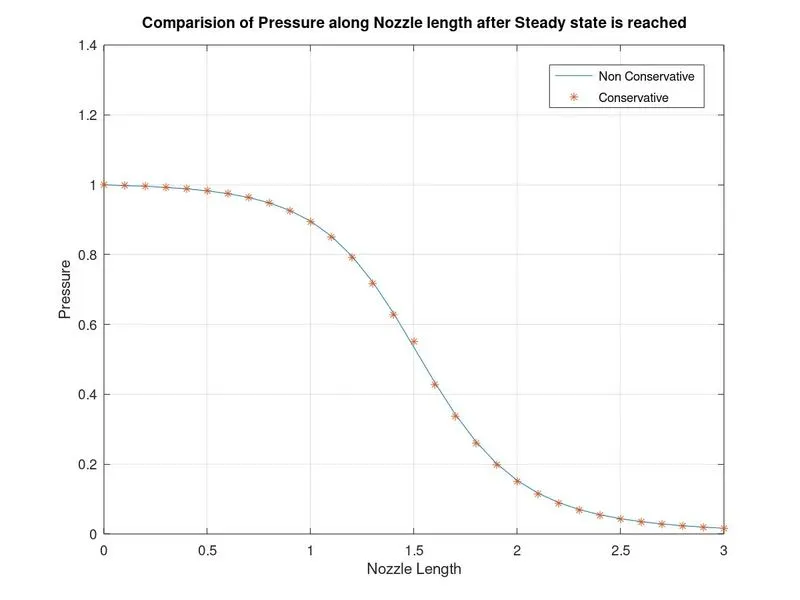
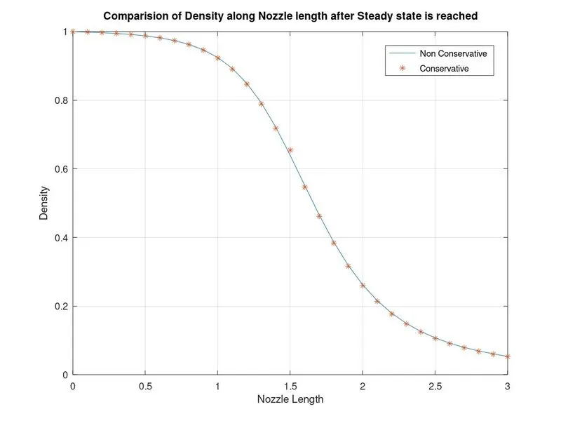
Comparision of Variation of Non-Dimensional Mach Number,Pressure,Density and Temperature along the Nozzle

Comparision of Steady-state Distribution of Primitive variables inside the Nozzle

Comparining non-dimensional Mach Number

Comparining non-dimensional Pressure

Comparining non-dimensional Density

Comparining non-dimensional Temperature

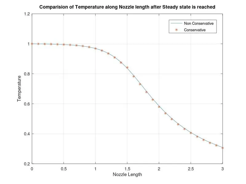
From the above plots it can be said that once the solution converges in both forms, the Primitive variables are almost same along the nozzle in both the forms. It almost looks like the variables obtained from conservative and non conservative form are equal at all points along the nozzle althought closer look may yield some differences.

It can be finally concluded from all the comparisions and studies made, both conservative form and non conservative form of governing equations produce good solution when MacCormack method is employed to simulate the isentropic flow in 1-D supersonic nozzle. One form is better than other in some of the aspects but when simulated for 1400 time steps with CFL=0.5 and with given initial and boundary conditions, the final solutions obatined for different primitive variables are accepted and are almost near to the exact analytical values. Assuming the other CFL number near to 1, the dt will change, so the solutions obtained may vary(may improve also) but for our case of CFL=0.5, solutions obtained from both conservative and non conservative form are satisfactory for both nodes n=31 and n=61. So employing MacCormack method for simulating 1D supersonic nozzle with time marching procedure yields good results for both forms of governing equations making the method good one.