Week 11 - Simulation of Flow through a pipe in OpenFoam
Aim:
To simulate an axi-symmetric flow by applying the wedge boundary condition for a laminar flow through a constant cross-section pipe at an inlet Reynold's number of 2100 and validate results with the Hagen- Poiseuille's equations for the fully developed flow.
To write code in Matlab to automate the generation of blockMeshDict file with inputs like pipe length, diameter, wedge angle, etc.
Hydrodynamic Entrance Length
The entrance length is the distance a flow travels after entering a pipre before the flow becomes fully developed. Entrance length refers to the length of the entry region, the area following the pipe entrance where effects originating from the interior wall of the pipe propagate into the flow as an expanding boundary layer. When the boundary layer expands to fill the entire pipe, the developing flow becomes a fully developed flow, where flow characteristics no longer change with increased distance along the pipe.
Hydrodynamic entrance length describes the formation of a velocity profile caused by viscous forces propagating from the pipe wall.
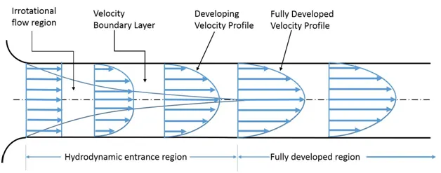
The hydrodynamic entrance region refers to the area of a pipe where fluid entering a pipe develops a velocity profile due to viscous forces propagating from the interior wall of a pipe. This region is characterized by a non-uniform flow. The fluid enters a pipe at a uniform velocity, then fluid particles in the layer in contact with the surface of the pipe come to a complete stop due to the no slip condition( the no-slip condition for viscous fluids assumes that at a solid boundary, the fluid will have zero velocity relative to the boundary). Due to viscous forces within the fluid, the layer in contact with the pipe surface resists the motion of adjacent layers and slows adjacent layers of fluid down gradually, forming a velocity. The velocity of layers of the fluid in the center of the pipe increases to compensate for the reduced velocities of the layers of fluid near the pipe surface. This develops a velocity gradient across the cross section of the pipe.
Hydrodynamic Entrance length is a function of Reynolds number of the flow. The Reynolds number is the ratio of inertial forces to viscous forces within a fluid which is subjected to relative internal movement due to different fluid velocities.
Laminar flow occurs at low Reynolds numbers, where viscous forces are dominant, and is characterized by smooth, constant fluid motion. Usually the flow is said to be laminar if the Reynold’s number is below 2300 and transition regime is between 2300 and 4000 and the flow becomes turbulent if Reynold’s number is greater than 4000.
Hagen-Poiseuille Equation
The Hagen–Poiseuille equation, is a law that gives the pressure drop in an incompressible fluid in laminar flow flowing through a long cylindrical pipe of constant cross section. The flow is laminar through a pipe of constant circular cross-section that is substantially longer than its diameter; and there is no acceleration of fluid in the pipe.
The equation is given by
`Deltap = (32 * mu * L * V_(avg) )/(D)^2`
Where
`mu` is the dynamic Viscosity of water
L is the hydrodynamic entrance length of the pipe and is given by
`L_e = (0.06 * R * D)`
R is the Reynolds number and is given by
`R = (V_(avg) * D)/ nu`
`nu` is the kinematic viscosity of the fluid is the ratio of dynamic viscosity to the density pf the fluid.
`nu = mu / rho`
So Reynolds number can also be written as
`R = (rho * V_(avg) * D) / mu`
Where V_avg is the average velocity of the fluid inside the pipe and is given by
`V_(avg) = ( R * mu)/(rho*D) = (R * nu)/D`
and D is the diameter of the pipe and is taken as 0.02 m for thr current simulation.
Reynolds number of the flow is considered to be 2100 which makes the flow laminar for the current simulation.
Equations and Analytical solutions from HP equation for the Simulation
Assumptions made are
- Flow is steady, incompressible (density is constant) and laminar.
- Constant fluid properties like Viscosity and density
Entry length for laminar flow, `L_e = (0.06 * R * D)`
Diameter of pipe D = 0.02 m
Given
At `25^0` C,
Density of the water - 997 `(kg)/m^3`
Water is taken as the working fluid
Kinematic Viscosity `nu = mu / rho` = 0.8917e-6 `m^2/s`
Dynamic Viscosity `mu = nu * rho` = (997) * (0.8917e-6) = 0.889e-3 poise
Reynolds number `R = (rho * V_(avg) * D) / mu`
R = 2100
Average Velocity `V_(avg) = mu *R/(rho*D)` = (0.889e-3*2100)/(997*0.02) = 0.0936 m/s
Maximum Velocity V_max = 2 * V_avg = 2 * 0.0936 = 0.18726 m/s
Hydrodynamic Length `L_e = (0.06 * R * D)` = 0.06 * 2100 * 0.02 = 2.52 m
From Hagen–Poiseuille equation, pressure drop is
`Deltap = (32 * mu * L * V_(avg) )/(D)^2` = 32 * 0.889e-3 * 0.09368 * 2.52/(0.02)^2 = 16.79 Pa
Kinematic pressure which is the pressure used at boundary condition in incompressible flows in openFoam is
Kinematic pressure `P = (Deltap)/rho` = 16.79/997 = 0.01684 `m^2/s^2`
The theta value for the wedge is varied and all these values for flow through the pipe are calculated accordingly in MATLAB and these values are used in the OpenFOAM to simulate the flow.
Simulating the flow in OpenFOAM
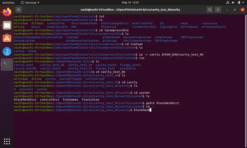
Start in the new terminal and surf to the tutorial folder by typing ‘tut’ to view the inbuilt tutorials in openFOAM.
We can see the list of folders inside any folder by typing in ls. Then we have to navigate to the incompressible folder by using ‘cd incompressible’ which changes the directory to incompressible folder.
The required flow can be simulated using the icoFoam solver. So in incompressible we navigate to icoFoam and there we choose the cavity folder.
Then this cavity folder is copied to the run folder by making use of ‘cp –r cavity $FOAM_RUN/cavity_test_06 (The user defined name). All these steps can be seen in the below figure.
Creating the blockMeshDict
The blockMeshDict for the flow is changed according to the required geometry and is created in the MATLAB by making use of file parsing techniques and making use of fopon and fclose commands and the required values are written into the f1 folder by using ‘w’ command which means write in to the f1 folder.
The all required inputs are given and the vertices V0 to V5 are calculated, the required angle theta is taken as user defined input and header of the blockMeshDict are defined and finally the faces, edges, arcs, wall, inlet and outlet of the wedge are created.
After defining the vertices of the wedge, the block is created. hex creates the hexahedral mesh and list of vertices are given. The first and second vertices represent the local x- axis, second and third vertices represent local y axis and next vertices is defined such that these four vertices defines the xy plane making the local z-axis perpendicular to this plane. The next four vertices are defined in the same manner but at a certain distance.
For discretization, in the next parenthesis the number of mesh points or cells are defined along the axes.
In simpleGrading is used for mesh stretching. Mesh grading factor f is the ratio of size of the end cell to the size of the staring cell and it makes the mesh finer at the required place and increases the meshing efficiency. Mesh grading 0.2 is used along x-axis which makes the size of the end cell 0.2 times the size of the starting cell along x-axis and mesh grading 1 is used for other 2 axes.
Next the axis of the flow is defined in the direction from vertex 0 to 3 the type of the boundary is empty. Wall is defined in order of vertices (2 5 4 1 ) in counter clockwise direction when viewed the wedge from outside and ‘wall’ type boundary is given for this face and no slip condition will be given for this wall. For the inlet the face (0 2 1 0) is taken in counter clockwise direction and patch type condition is given for this inlet face. Order of vertices naming is clockwise for the outlet as it is viewed from the inside the geometry and patch type face is given for outlet. Front face (0 3 5 2) is named in counter clockwise direction and back face in clockwise and wedge type boundary condition is given for these faces.
Upon describing all these in MATLAB, the blockMeshDict file is created for the given theta and this file will replace the default blockMeshDict in the system folder of the cavity in icoFoam of incompressible folder in openFoam tutorials.
Then the mesh using this blockMeshDict is created by using command blockMesh and mesh accuracy is checked using command checkMesh.
Then the kinematic pressure and average velocity values calculated for the given theta will be used at the outlet and inlet of the geometry respectively.
The blockMeshDict.txt file is created using the following MATLAB code.
MATLAB Code:
    clear all
    close all
    clc

    %Simulation of Laminar Flow Through Pipe

    %Inputs
    Rey = 2100;    %Reynold's Number
    dia = 0.02;     %Diameter of the Pipe
    rho = 997;    %Density of the Water
    mu = 0.89e-3   %Dynamic Viscosity of Water
    nu = mu/rho    %Kinematic Viscosity of Water
    r = dia/2    %Radius of the Pipe

    %Hydrodynamic Entrance Length of the Pipe
    L = 0.06 * Rey * dia

    V_avg = (Rey * nu )/ dia     %Avearge Velocity
    V_max = 2 * V_avg            %Maximum Velocity

    %Pressure difference
    dp = (32 * mu * L * V_avg) / (dia ^ 2)

    %Kinematic Pressure which is the BC at the outlet
    kine_pressure = dp/rho

    theta = input('Enter the value of Theta = ')   %Value should be less than 5

    %Calculating Vortices
    V0 = [ 0 0 0]
    V1 = [ 0 r*cosd(theta/2) -r*sind(theta/2) ]
    V2 = [ 0 r*cosd(theta/2) r*sind(theta/2) ]

    V3 = [ L 0 0]
    V4 = [ L r*cosd(theta/2) -r*sind(theta/2) ]
    V5 = [ L r*cosd(theta/2) r*sind(theta/2) ]

    s1 = blanks(4)
    s2 = blanks(8)
    s3 = blanks(12)

    %Creating blockMeshDict File for openFOAM

     %Header Information
     h1 =  '  /*--------------------------------*- C++ -*----------------------------------*\'
     h2 = '========= |'
     h3 = '\\      /  F ield | OpenFOAM: The Open Source CFD Toolbox'
     h4 = ' \\    /   O peration | Website: https://openfoam.org'
     h5 = '  \\  /    A nd | Version: 8'
     h6 = '   \\/     M anipulation |'
     h7 = '\*---------------------------------------------------------------------------*/'
     h8 = 'FoamFile'
     h9 = '{'
     h10 = 'version 2.0;'
     h11 = 'format ascii;'
     h12 = 'class dictionary;'
     h13 = 'object blockMeshDict;'
     h14 = '}'
     h15 = '// * * * * * * * * * * * * * * * * * * * * * * * * * * * * * * * * * * * * * //'

     f1 = fopen('blockMeshDict.txt','w');   %Writing into blockMeshDict file with text extension
     fprintf(f1,'%s \n',h1)
     fprintf(f1,'%s \n',h2)
     fprintf(f1,'%s \n',h3)
     fprintf(f1,'%s \n',h4)
     fprintf(f1,'%s \n',h5)
     fprintf(f1,'%s \n',h6)
     fprintf(f1,'%s \n',h7)
     fprintf(f1,'%s \n',h8)
     fprintf(f1,'%s \n',h9)
     fprintf(f1,'%s \n',h10)
     fprintf(f1,'%s \n',h11)
     fprintf(f1,'%s \n',h12)
     fprintf(f1,'%s \n',h13)
     fprintf(f1,'%s \n',h14)
     fprintf(f1,'%s \n',h15)
     fprintf(f1,'\n')

     fprintf(f1,'%s \n','convertToMeters 1;')
     fprintf(f1,'\n')

     axis = '(0 3 3 0)'
     wall = '(2 5 4 1)'
     inlet = '(0 2 1 0)'
     outlet = '(3 4 5 3)'
     front = '(0 3 5 2)'
     back = '(0 1 4 3)'

     %Vertices
     fprintf(f1,'%s \n','vertices')
     fprintf(f1,'%s \n','(')
     fprintf(f1,'%s (%d %d %d) \n',s1, V0(1),V0(2),V0(3))
     fprintf(f1,'%s (%d %d %d) \n',s1, V1(1),V1(2),V1(3))
     fprintf(f1,'%s (%d %d %d) \n',s1, V2(1),V2(2),V2(3))
     fprintf(f1,'%s (%d %d %d) \n',s1, V3(1),V3(2),V3(3))
     fprintf(f1,'%s (%d %d %d) \n',s1, V4(1),V4(2),V4(3))
     fprintf(f1,'%s (%d %d %d) \n',s1, V5(1),V5(2),V5(3))
     fprintf(f1,'%s \n',');')
     fprintf(f1,'\n')

     %blocks
     fprintf(f1,'%s \n','blocks')
     fprintf(f1,'%s \n','(')
     fprintf(f1,'%s hex (0 1 2 0 3 4 5 3) (50 1 200) simpleGrading (0.2 1 1)\n',s1)
     fprintf(f1,'%s \n',');')
     fprintf(f1,'\n')

     %Edges
     fprintf(f1,'%s \n','edges')
     fprintf(f1,'%s \n','(')
     fprintf(f1,'%s %s %d %d (%d %d %d) \n',s1,'arc',1,2,0,r,0)
     fprintf(f1,'%s %s %d %d (%d %d %d) \n',s1,'arc',4,5,L,r,0)
     fprintf(f1,'%s \n',');')
     fprintf(f1,'\n')

     %Boundary
     fprintf(f1,'%s \n','boundary')
     fprintf(f1,'%s \n','(')

     %axis
     fprintf(f1,'%s %s \n',s1,'axis')
     fprintf(f1,'%s %s \n',s1,'{')
     fprintf(f1,'%s %s \n',s2,'type empty;')
     fprintf(f1,'%s %s \n',s2,'faces')
     fprintf(f1,'%s %s \n',s2,'(')
     fprintf(f1,'%s %s \n',s3,axis)
     fprintf(f1,'%s %s \n',s2,');')
     fprintf(f1,'%s %s \n',s1,'}')
     fprintf(f1,'\n')

     %Wall
     fprintf(f1,'%s %s \n',s1,'wall')
     fprintf(f1,'%s %s \n',s1,'{')
     fprintf(f1,'%s %s \n',s2,'type wall;')
     fprintf(f1,'%s %s \n',s2,'faces')
     fprintf(f1,'%s %s \n',s2,'(')
     fprintf(f1,'%s %s \n',s3,wall)
     fprintf(f1,'%s %s \n',s2,');')
     fprintf(f1,'%s %s \n',s1,'}')
     fprintf(f1,'\n')

     %Inlet
     fprintf(f1,'%s %s \n',s1,'inlet')
     fprintf(f1,'%s %s \n',s1,'{')
     fprintf(f1,'%s %s \n',s2,'type patch;')
     fprintf(f1,'%s %s \n',s2,'faces')
     fprintf(f1,'%s %s \n',s2,'(')
     fprintf(f1,'%s %s \n',s3,inlet)
     fprintf(f1,'%s %s \n',s2,');')
     fprintf(f1,'%s %s \n',s1,'}')
     fprintf(f1,'\n')


     %Outlet
     fprintf(f1,'%s %s \n',s1,'outlet')
     fprintf(f1,'%s %s \n',s1,'{')
     fprintf(f1,'%s %s \n',s2,'type patch;')
     fprintf(f1,'%s %s \n',s2,'faces')
     fprintf(f1,'%s %s \n',s2,'(')
     fprintf(f1,'%s %s \n',s3,outlet)
     fprintf(f1,'%s %s \n',s2,');')
     fprintf(f1,'%s %s \n',s1,'}')
     fprintf(f1,'\n')


     %Front
     fprintf(f1,'%s %s \n',s1,'front')
     fprintf(f1,'%s %s \n',s1,'{')
     fprintf(f1,'%s %s \n',s2,'type wedge;')
     fprintf(f1,'%s %s \n',s2,'faces')
     fprintf(f1,'%s %s \n',s2,'(')
     fprintf(f1,'%s %s \n',s3,front)
     fprintf(f1,'%s %s \n',s2,');')
     fprintf(f1,'%s %s \n',s1,'}')
     fprintf(f1,'\n')


     %Back
     fprintf(f1,'%s %s \n',s1,'back')
     fprintf(f1,'%s %s \n',s1,'{')
     fprintf(f1,'%s %s \n',s2,'type wedge;')
     fprintf(f1,'%s %s \n',s2,'faces')
     fprintf(f1,'%s %s \n',s2,'(')
     fprintf(f1,'%s %s \n',s3,back)
     fprintf(f1,'%s %s \n',s2,');')
     fprintf(f1,'%s %s \n',s1,'}')
     fprintf(f1,'%s \n',');')
     fprintf(f1,'\n')


     fprintf(f1,'\n')
     fprintf(f1,'%s \n','mergePatchPairs')
     fprintf(f1,'%s \n','(')
     fprintf(f1,'%s \n',');')
     fprintf(f1,'\n')
     fprintf(f1,'%s \n',h15)
     fprintf(f1,'\n')

     fclose(f1)
The blockMeshDict file for the simulation for wedge angle 4° is given below.
  /*--------------------------------*- C++ -*----------------------------------*\
========= |
\\      /  F ield | OpenFOAM: The Open Source CFD Toolbox
 \\    /   O peration | Website: https://openfoam.org
  \\  /    A nd | Version: 8
   \\/     M anipulation |
\*---------------------------------------------------------------------------*/
FoamFile
{
version 2.0;
format ascii;
class dictionary;
object blockMeshDict;
}
// * * * * * * * * * * * * * * * * * * * * * * * * * * * * * * * * * * * * * //

convertToMeters 1;

vertices
(
     (0 0 0)
     (0 0.00999391 -0.000348995)
     (0 0.00999391 0.000348995)
     (2.52 0 0)
     (2.52 0.00999391 -0.000348995)
     (2.52 0.00999391 0.000348995)
);

blocks
(
     hex (0 1 2 0 3 4 5 3) (50 1 200) simpleGrading (0.2 1 1)
);

edges
(
     arc 1 2 (0 0.01 0)
     arc 4 5 (2.52 0.01 0)
);

boundary
(
     axis
     {
         type empty;
         faces
         (
             (0 3 3 0)
         );
     }

     wall
     {
         type wall;
         faces
         (
             (2 5 4 1)
         );
     }

     inlet
     {
         type patch;
         faces
         (
             (0 2 1 0)
         );
     }

     outlet
     {
         type patch;
         faces
         (
             (3 4 5 3)
         );
     }

     front
     {
         type wedge;
         faces
         (
             (0 3 5 2)
         );
     }

     back
     {
         type wedge;
         faces
         (
             (0 1 4 3)
         );
     }
);


mergePatchPairs
(
);

// * * * * * * * * * * * * * * * * * * * * * * * * * * * * * * * * * * * * * //
Next the inlet and outlet boundary conditions are given for the flow. At the inlet the velocity of the flow is given which is the constant value and the value is given from the calculated average value from the MATLAB code and this value is U = 0.0937m/s along x-axis and along other 2 axes valuie is kept as 0.
No slip condition is given for the wall and at other faces zeroGradient is given. All these changes are made in the ‘0’ folder which holds in initial condition values i.e., at time t=0. In ‘0’ folder, the U is edited by using the command gedit U and the necessary changes are made and values are assigned at different faces as mentioned above.
The pressure field is simulated by using command gedit p and the kinematic pressure which is calculated from the code is used in the incompressible flow simulation. This kinematic pressure is given at the outlet of the geometry and the value is p = 0.0168 `m^2/s^2`. At wall and the inlet the zeroGradient condition is given for pressure.
And at front and back faces, wedge type boundary condition is given in both p and U folders.
Next in the controlDict folder the starting time, the time step and the end time are described. Simulation is run for 5 seconds with time step 0.01 keeping in mind the necessary CFL numbers in the required range to make the solution stable.
Next the nu which is kinematic viscosity of the fluid calculated from the code is specified in the transport properties of the constant folder.
Then the simulation is ran with the command ‘icoFoam’ which is the name of the solver and the result of the simulation is viewed using ‘paraFoam’ command for post-processing procedures.
Boundary Conditions:
Velocity(U) - (Inlet):
/*--------------------------------*- C++ -*----------------------------------*\
  =========                 |
  \\      /  F ield         | OpenFOAM: The Open Source CFD Toolbox
   \\    /   O peration     | Website:  https://openfoam.org
    \\  /    A nd           | Version:  8
     \\/     M anipulation  |
\*---------------------------------------------------------------------------*/
FoamFile
{
    version     2.0;
    format      ascii;
    class       volVectorField;
    object      U;
}
// * * * * * * * * * * * * * * * * * * * * * * * * * * * * * * * * * * * * * //

dimensions      [0 1 -1 0 0 0 0];

internalField   uniform (0.0937 0 0);

boundaryField
{
     axis
    {
        type            empty;
    }

    wall
    {
        type            noSlip;
    }

     inlet
    {
        type            fixedValue;
        value           uniform (0.0937 0 0);
    }

     outlet
    {
        type            zeroGradient;
    }

     front
    {
        type            wedge;
    }

     back
    {
        type            wedge;
    }
}

// ************************************************************************* //
Kinematic Pressure(p) - (Outlet):
/*--------------------------------*- C++ -*----------------------------------*\
  =========                 |
  \\      /  F ield         | OpenFOAM: The Open Source CFD Toolbox
   \\    /   O peration     | Website:  https://openfoam.org
    \\  /    A nd           | Version:  8
     \\/     M anipulation  |
\*---------------------------------------------------------------------------*/
FoamFile
{
    version     2.0;
    format      ascii;
    class       volScalarField;
    object      p;
}
// * * * * * * * * * * * * * * * * * * * * * * * * * * * * * * * * * * * * * //

dimensions      [0 2 -2 0 0 0 0];

internalField   uniform 0;

boundaryField
{
    axis
    {
        type            empty;
    }

    wall
    {
        type            zeroGradient;
    }

     inlet
    {
        type            zeroGradient;
    }

     outlet
    {
        type            fixedValue;
        value           uniform 0.01686;
    }

     front
    {
        type            wedge;
    }

     back
    {
        type            wedge;
    }
}

// ************************************************************************* //
controlDict file:
/*--------------------------------*- C++ -*----------------------------------*\
  =========                 |
  \\      /  F ield         | OpenFOAM: The Open Source CFD Toolbox
   \\    /   O peration     | Website:  https://openfoam.org
    \\  /    A nd           | Version:  8
     \\/     M anipulation  |
\*---------------------------------------------------------------------------*/
FoamFile
{
    version     2.0;
    format      ascii;
    class       dictionary;
    location    "system";
    object      controlDict;
}
// * * * * * * * * * * * * * * * * * * * * * * * * * * * * * * * * * * * * * //

application     icoFoam;

startFrom       startTime;

startTime       0;

stopAt          endTime;

endTime         5;

deltaT          0.01;

writeControl    timeStep;

writeInterval   100;

purgeWrite      0;

writeFormat     ascii;

writePrecision  6;

writeCompression off;

timeFormat      general;

timePrecision   6;

runTimeModifiable true;


// ************************************************************************* //
transportProperties file:
/*--------------------------------*- C++ -*----------------------------------*\
  =========                 |
  \\      /  F ield         | OpenFOAM: The Open Source CFD Toolbox
   \\    /   O peration     | Website:  https://openfoam.org
    \\  /    A nd           | Version:  8
     \\/     M anipulation  |
\*---------------------------------------------------------------------------*/
FoamFile
{
    version     2.0;
    format      ascii;
    class       dictionary;
    location    "constant";
    object      transportProperties;
}
// * * * * * * * * * * * * * * * * * * * * * * * * * * * * * * * * * * * * * //

nu              [0 2 -1 0 0 0 0] 0.892e-6;


// ************************************************************************* //
Outputs and Results:
The vertices for the wedge angle 4° for diameter 0.02m is
V0 = [ 0 0 0]
V1 = [0.0000000 0.0099939 -0.0003490]
V2 = [ 0.0000000 0.0099939 0.0003490]
V3 = [ 2.52000 0.00000 0.00000]
V4 = [ 2.52000000 0.00999391 -0.00034899]
V5 =[ 2.52000000 0.00999391 0.00034899]
So the hydrodynamic entrance length of the pipe is 2.52m which means the flow is fully developed at this distance from the inlet and the flow properties do not change much with increased distance along the pipe.
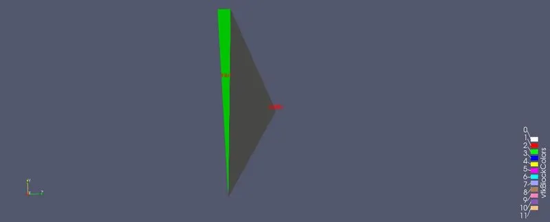
The geometry for wedge angle 4° looks as below. We can see the inlet of the geometry with given 4° wedge angle with wall on top if the geometry. It also has outlet on the other side.
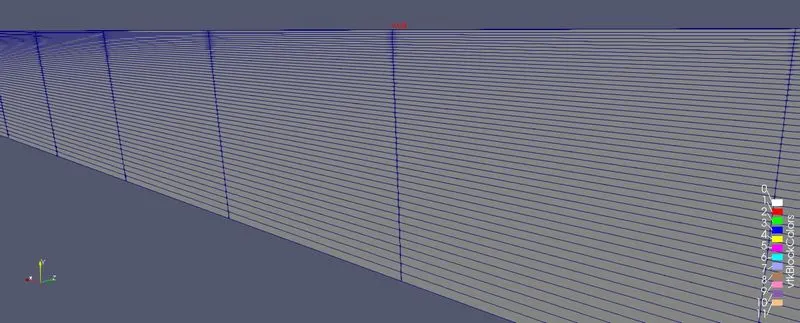
Meshing of the domain for grading factor 0.2 is shown below.
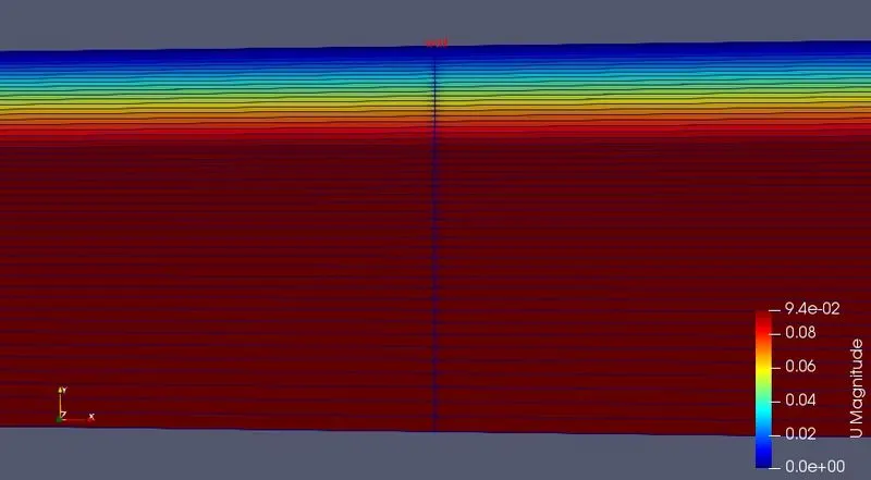
The velocity profile along the pipe with velocity varying from the wall to the centre of the pipe. Here we can see that at any distance from the inlet, along the radius of the pipe, the velocity is very less or 0 at the wall section of the pipe due to assumed no slip condition. Velocity increases when we move from wall towards the centre and the same trend is followed at any distance from the inlet. In order to compensate for the less velocity at the wall, the velocity is higher at the centre and from the centre as we move towards the opposite wall, the velocity decreases and becomes zero again at the wall section. So we can say the velocity profile is symmetric to the axis.
The velocity profile at dvarious distances from the Inlet:
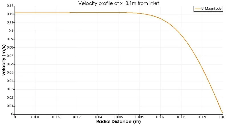
At 0.1m from the inlet, the velocity across the radial distance will be lesser and is around 0.123m/s and here also the velocity at the wall can be seen as zero and the maximum velocity is at the centre i.e., r=0 and the velocity is constant till r = 0.07 and reduces suddenly. So we can say the reduction in velocity is not so linear as the velocity is not developed.
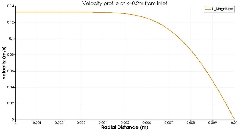
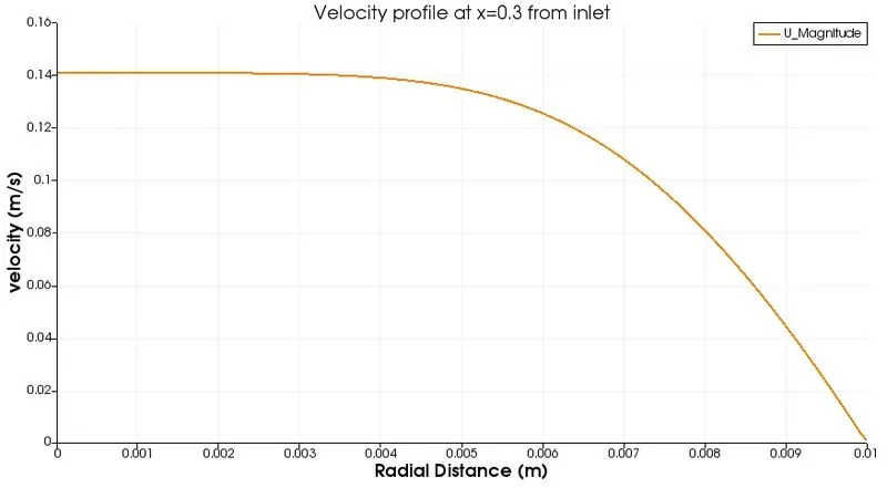
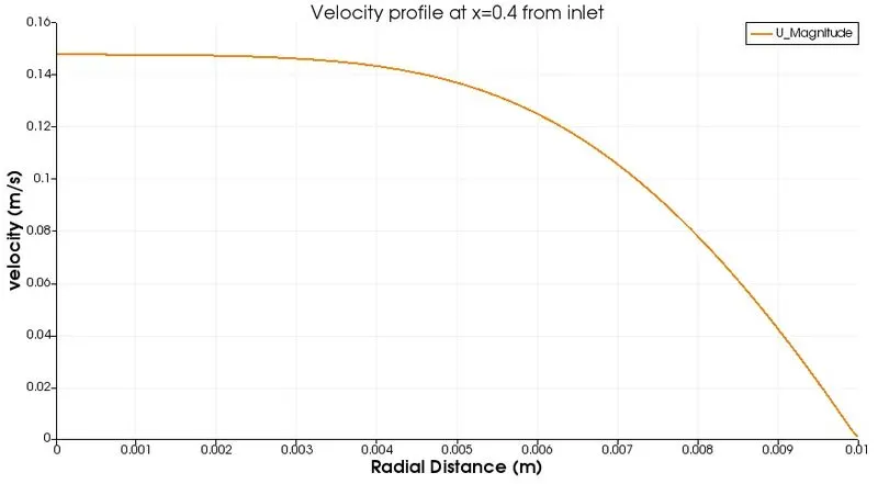
From above 3 graphs we can see that the maximum velocity is increasing with the increase in the distance and also the reduction in the velocity along the radial distance is also not sudden and we can say that there is a improvement in the velocity profile.
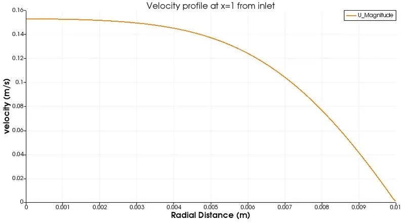
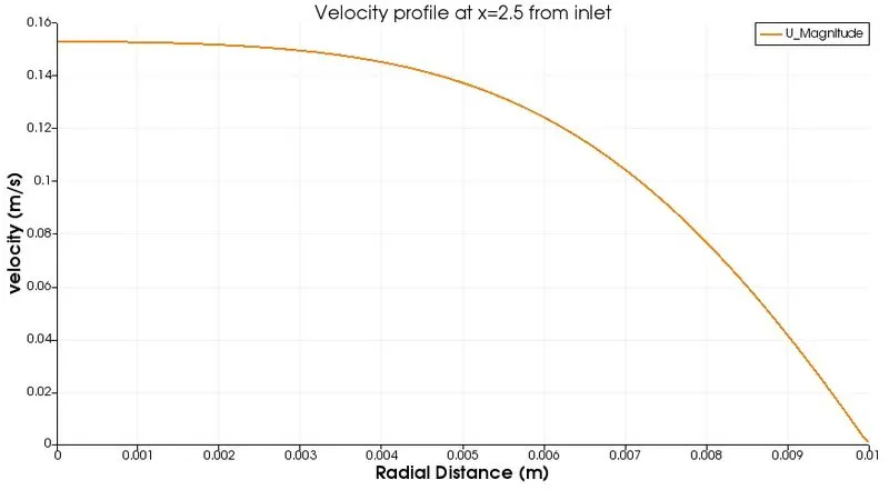
We can see from the above graphs that the the maximum velocity is around 0.158 or 0.16m/s and the maximum velocity from our analytical calculation is 0.18m/s. So we can say there is a match between the analytical solution and our simulation. The some error in the maximum velocity corresponds to some considered assumptions and the given wedge angle. With the change in the wedge angle, there may be the possibility of the reduction in this error but we can say from our simulation the results are satisfactory for maximum velocity.
And also the reduction in the velocity along radial distance can also be seen as somewhat linear and reduction is not sudden as in the case at near the inlets due to the development of boundary layer adjacent to the wall which slows down the velocity of fluid in that region.
Also from the inlet distance x=2m and x=2.5m we can see that the velocity profiles do not vary much. So we can say that the hydrodyanamic entrance region will be between these values. So we can say tge hydrodyamic entrance region from out simulation can be said as 2.5m as there will not be any major changes in the velocity profile with the increase in the distance from the inlet. From analytical solution also this length is 2.52m . So as there is no much change in the velocity profiles, now we can say that our flow is fully developed within the hydrodynamic entrance region and these values are identical to our analytical solutions.
Shear Stress:
The shear stress `tau` is highest at the pipe inlet, where the boundary layer thickness is the smallest. Shear stress decreases along the flow direction. That is why the pressure drop is highest in the entrance region of a pipe.
Analytically it can be calculated as :
`tau = mu (du)/(dy)`
- `tau` is the dynamic viscosity of the flow and here it is 0.89e-3
- `(du)/(dy)` is the shear deformation
By using maximum velocity shear stress can be calculated at a certain distance from the inlet or at a distance where maximum velocity occurs as below.
    clear all
    close all
    clc

    %Simulation of Laminar Flow Through Pipe
    %Shear Stress

    %Inputs
    Rey = 2100;    %Reynold's Number
    dia = 0.02;     %Diameter of the Pipe
    rho = 997;    %Density of the Water
    mu = 0.89e-3   %Dynamic Viscosity of Water
    nu = mu/rho    %Kinematic Viscosity of Water
    r = dia/2    %Radius of the Pipe
    V_avg = (Rey * nu )/ dia     %Avearge Velocity
    V_max = 2 * V_avg            %Maximum Velocity

    R = linspace(0,r,100)

    shear_stress = (2 * mu * V_max .* R)./(r^2)

    %Plotting
    plot(R,shear_stress,'r','linew',2)
    xlabel('Radial Distance in m')
    ylabel('Shear Stress in N/m^2')
    grid on
    title('Variation of Shear Stress along Radial length for fully developed Flow')
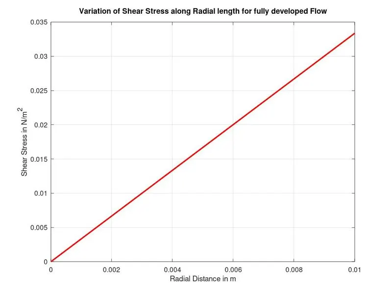
At the wall of the pipe, velocity of the fluid will be zero. In the adjacent layer to the wall, since there is a motion of the fluid, friction between them creates force and subsequently the shear stress. So due this shear stress set up in larger values at the boundary layer and wall of the pipe at any region of pipe. Also shear stress are high at the inlet of the pipe and reduces as the flow propogates in the pipe.
Conclusions:
From the plots we can see that velocity profile increases from inlet to the outlet (from x=0 to x=2.8m). Velocity profile tends to increase slowly with increase in distance along the pipe and reaches the maximum velocity at the outlet. This is the region we call as a fully developed region as we can see velocity profile develops completely at the outlet section.
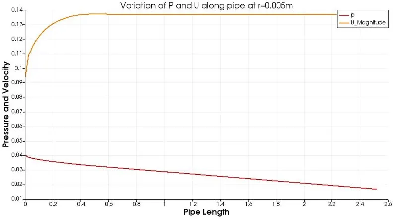
However at walls velocity remains zero along the length of the pipe due to the assumed or applied no slip boundary condition. And also along the pipe , there is a formation of boundary layer adjacent to the wall which slows down the flow near to the. In order to compensate for this reduction the velocity the centre goes on increasing and finally at the outlet we can see the velocity somewhat increasing linearly from wall to the centre and we can say the velocity profile is fully developed and it obeys the hagen Poiseuilles’s law to fully develop within the analytical hydrodynamic entrance length. From velocity and pressure plot along the pipe at r=0.005 from centre, we can see the pressure is getting dropped and at the same time velocity being increased along the length of the pipe.
So we can say that the domain and the mesh generated for wedge angle = 4° simuates the flow along the pipe with the given boundary conditions and it obeys the Hagen Poiseuille’s equation and the velocity profile is proved to be fully developed from the above plots and there will be pressure drop and increase in velocity along the pipe length.