Week 4.2: Project Transient simulation of flow over a throttle body
Aim:
To simulate the flow over the throttle inside the elbow and to study pressure, velocity contours and plots for pressure, velocity, mass flow rate and total cell count. The simulation is the transient simulation and the throttle should rotate inside the elbow for the specified time.
Throttle:
A throttle is the mechanism by which fluid flow is managed by constriction or obstruction. An engine's power can be increased or decreased by the restriction of inlet gases by the use of a throttle. The throttle refers to any mechanism by which the power or speed of an engine is regulated, such as a car's accelerator pedal. In the current simulation the throttle is rotated by an angle of 25 degree for first 2 milli seconds, kept at that poistion for 2 more milli seconds, then brought back to origions position in 4 ms. Transient simulation is carried out to perfirm this simulation of throttle movement in Convegre software and variation of fluid flow quantities at the throttle are studied.
Simulation Process:
Import the file of geometry of the elbow in STL extension into Converge.
Delete the thickness of the geometry and patch the thus formed open edges in the geometry. The scale of 0.001 is provided to the geometry to convert it into mms.
Run diagnosis and if there are any normals orientating outside the geometry, then go to transform, noraml and select any triangle and hit apply. All normals should be pointing inwards.
Then go to boundary > Flag and select create multiple boundaries.
Geometry clean up and Boundary Flagging:
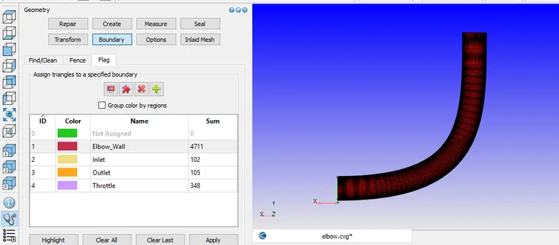
Above figure shows the geometry of the elbow with the throttle inside it. Geometry is flagged into inlet, outlet, elbow wall and the throttle. Throttle is used to maintain the rate of the flow inside the elbow and can be seen below
Dimensions of Geometry:
Lx = 0.106m
Ly = 0.119m
Lz = 0.017m
Visualisation of Throttle:
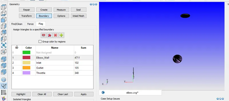
The centre part is the throttle placed inside the elbow along with inlet and outlet above and below it respectively.
Case Setup:
1. Applications type: Time - Based
2. Materials:
Select default values for Gas Simulation and Global Transport Properties and Select Air as Predefined Mixture
Species : Add N2 and O2 in Gas
as Air is the working fluid
3.Initial Condition and Events:
Add a region as Volumetric_Region in regions and Initialisation and intialise species value with below mass fraction
O2 - 0.23
N2 - 0.77 whose combination makes the Air as the working fluid for simulation.
4. Boundary Conditions:
Inlet
Boundary type - INFLOW.
Pressure - 150000 Pa
Temperature - 300 K
Species - N2 = 0.77 and O2 = 0.23
Outlet
Boundary type - OUTFLOW.
Pressure - 100000 Pa
Temperature - 300 K
Species - N2 = 0.77 and O2 = 0.23
This pressure difference between inlet and Outlet drives the flow from inlet and outlet .Also mention O2 and N2 species dor Backflow ( if it occurs due to adverse pressure)
Throttle
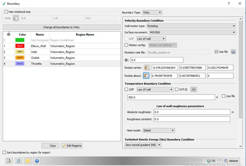
Since the throttle is rotated in this simulation
Boundary type - WALL
Wall motion : Rotating
Surface Movement : Moving
Apply Law of Wall for Velocity and Temperature Boundary Conditions.
To find out the Rotation Centre and Axis of rotation for throttle:
Hide the geometry of throttle except the two cyclinder like pieces
Go to Measure > Direction > Arc Normal and select three edges on the top surface so that we will be able to get the centre of that cylinder and the direction in which it is oriented and hit apply.
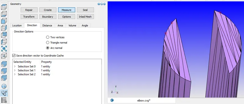
Then we will obtain the Arc Centre and ARC Normal Values. Copy and Paste them as Rotate Centre and Rotate about parameter in the Throttle boundary respectively. The vector values of Arc centre and Arc normal are (-0.0761543 0.03907780 0.0201742) and (0.7943977 0.607397 0) respectively.
Now for Rotate rate - check in Use file box and throttle rotation wrt time is specified.
Throttle Movement:
for 0-2ms throttle should rotate byan angle of 25 degrees
for 2-4ms throttle should remain at 25 degrees
for 4-8 ms throttle should come back to its initial position.
Mention the same values in the Rotate rate file and specify SEQUENTIAL type
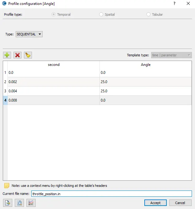
Save the file name as throttle_position.in
Specify Law of Wall for Velocity and Temperature Boundary coondition and finally our throttle boundary condition loojs as below.
Elbow_Wall
Boundary type - WALL
Wall motion : Stationary
Apply Law of Wall for Velocity and Temperature Boundary Conditions.
Select Volumetric_Region as Region name for all the boundaries since Volumetric_region is the region created for the boundaries.
5. Simulation Parameters:
Run parameters:
Solver : Transient
Simulation mode: Full hydrodynamic
Turn off use shared memory.
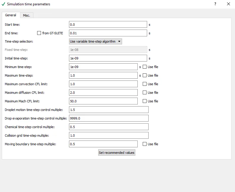
Simulation Time Parameters:
Start time - 0 seconds
Calculating end time for Simulation:
From the Steady state simulation, the velocity at the Inlet was around as 190 m/s for the provided initial conditions and Pressure of 150000 Pa and 100000 Pa at Inlet and outlet respectively. So since we are using the same pressure differnece, the velocity at the inlet can be considered as 190 m/s.
The maximum length of the elbow may be taken as 0.2 m since Lx = 0.106m and Ly = 0.119m. So keeping these values, time needed for the fluid to flow from inlet to outlet will be
`Speed = (distance )/ (time)`
so `time = (distance) / (speed)`
time = 0.2m / (190m/s) = 0.00105 seconds
and this time is called as Flow Through Time and here it is around 0.00105 seconds.
Simulation is ran for around 10 times of this flow through time to capture all required rotations of throttle. So
End time = 10 * Flow through time = 10 * 0.001 = 0.01 seconds.
End time - 0.01 seconds
Intial time step : 1e-9 s
Minimum time step:1e-9 s
Maximum Time step: 1 s
Maximum convection CFL limit: 1
Leave the rest as Default values.
And the same is shown in below figure
Solver Parameters:
N-S solver Scheme - PISO
N-S Solver Type - Pressure Based
6. Physical Models:
Turbulence model : RNG k -`epsilon` in RANS
7. Grid Control :
Base grid : dx=dy=dx = 0.002 m
Add fixed Embedding in Grid control
Fixed Embedding:
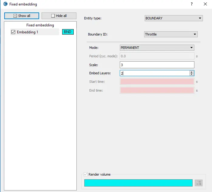
`Embedded Mesh size = (base mesh size) / (2^(SCALE)`
At the throttle major changes in the flow variables occur.. In Order to capture the results accurately at the throttle, fine mesh will be need with more cells. So mesh size is reduced at the throttle with the help of fixed embedding. Scale of 3 makes the reduces the base mesh size by 8(2^3) times and embedded lalayers 2 means the mesh size is further reduced by 8 times at the throttle boundary. So fixed embedding is provided at the Throttle boundary with Embed layers being 2 and scale of 3 using the PERMANENT mode.
8. Output/Post-processing
In post variable selection, under Species tab, add N2 and O2 in mass fraction box.
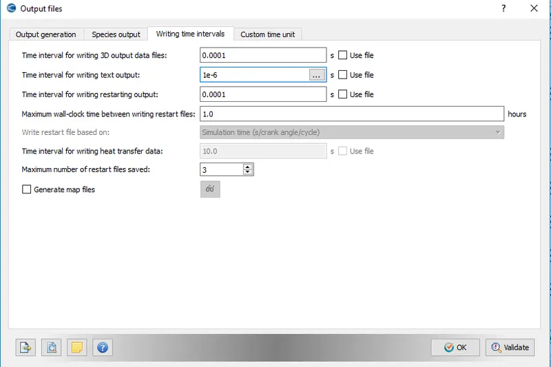
In output files, under Writing time intervals tab, in order to obtain 100 3D output files to cpature the results accurately, time interval for writing 3D output data files and restarting files is specified as 0.0001 sec since the end time is 0.01 seconds. 1e-6 sec is provided to time interval for writing text output so outputs are ibtained at each cycle of simulation.
Now Export All these input files to a directory. Open CYGWIN, navigate to the directory where all these folders are saved and run the following command ;
mpiexec.exe -n 4 converge.exe restricted logfile_006 &
which runs the simulation with 4 processors using converge executable and outputs are dumped into a file called logfile_006 with job being ran in backend.
Outputs/Post -Processing:
Post processing is performed in the paraview software using the group files with ..vtm extension created in the post processor of Converge
Geometry:
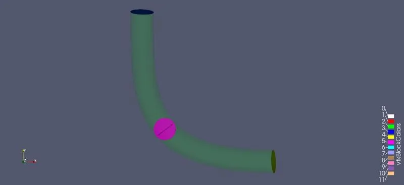
The geometry involving Throttle valve in pink color, inlet, outlet along with outer elbow can be seen.
Mesh:
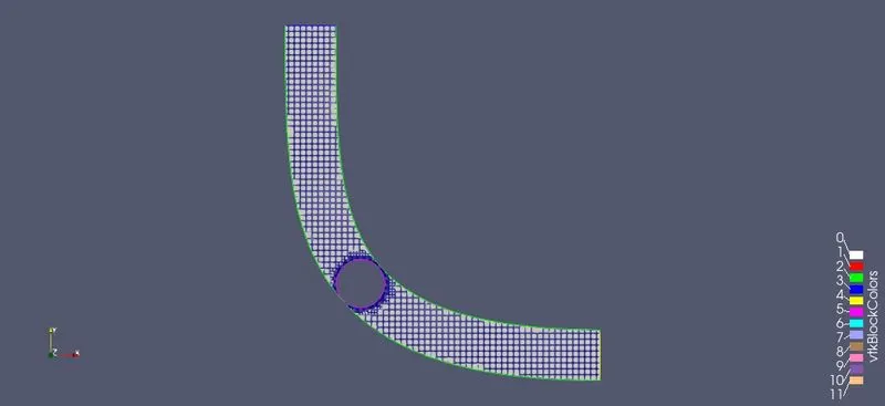
Finer Mesh at Throttle:
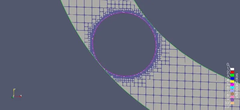
The finer mesh near throttle using the fixed embedding in order to obtain better results. The mesh on the complete geometry can be seen. This mesh is continuously changing in the simulation time due to the motion of the Throttle and this change of the mesh at throttle is shown in the below animation:
Animation of Mesh:
In the animation, the mesh near the throttle region can be seen increasing due change in the area of the throttle due to its rotation.
Pressure Contour:
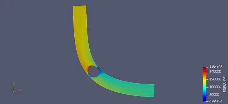
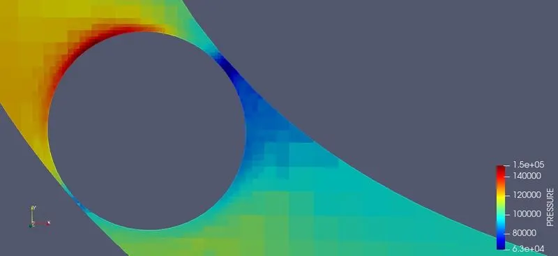
Since the flow will be stopped in front of the throttle, the kinetic energy converts into static pressure hence the increse in the static pressure can be seen. In the wake region where the flow rate will be less the static pressure decreases. above the throttle, where there is reduction in the area, the velocity increases reducing the pressure. The clear picture of the pressure distribution near throtlle can be seen in below pictures.
Pressure distribution near Throttle:
Animation of Variation of Pressure on the Throttle:
The following animations visualised the Pressure variation at the throttle from the start time to the end time of the simulation. Above the throttle, since the velocity will be increased due to reduction in area, pressure can be seen reducing. Also pressure at outlet is lesser than the same at the inlet. Also the rotation of the throttle inside the elbow for complete 0.01 seconds along with variation of pressure on it can be seen in below animations
When the throttle is at 25 degrees, blocking the flow in front of it, the pressure raised way high in front of it due to conversion of kinetic energy to pressure. When it again moves back to 0 degress, pressure reduces in the region before throttle. But at the throttle pressure always remains high since the some of the flow terminates.
Velocity Contour:
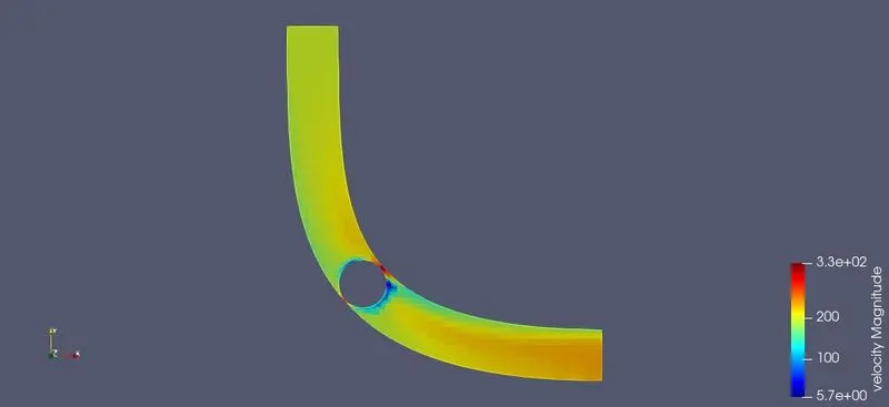
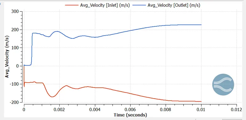
The velocity distribution at the outlet is higher than inlet. This is due to the reduction in the area near the throttle. The constriction of the area at the throttle makes the fluid drive at the faster velocity above the below the throttle. So the maximum velocity is produced near throttle. The velocity increase will also results in the increase of dynamic pressure and thus makes the compensation for reduction in static pressure.
Velocity distribution near Throttle:
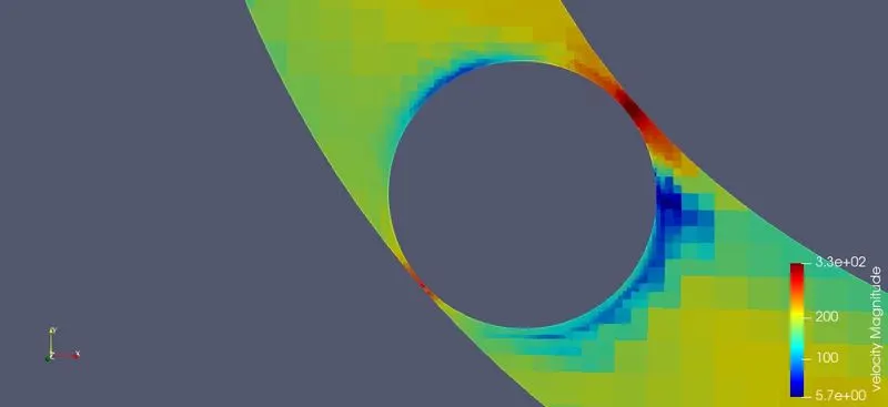
Velocity distribution near the throttle can be seen clearly in the above figure. Since there ist termination of flow due to the throttle, velocity is much lesser in that region. Also in wake region, where fluid flow is less, velocity is reduced. Velocity at the outlet is higher than inlet due to the reduction in the area for flow at throttle which increases the flow velocity. These are the values obtained at the end time of the transient simulation and the maximum Velocity inside the elbow is around 330m/s and occurs near the Throttle.
Animation of Variation of Velcoity on the Throttle:
The following animations visualised the Velocity variation at the throttle from the start time to the end time of the simulation. Above the throttle, since the velocity will be increased due to reduction in area. Also the rotation of the throttle inside the elbow for complete 0.01 seconds along with variation of velocity on it can be seen in below animations.
Velocity behind throttle is very low as there will be no flow in that region as throttle blocks the flow and the same can be seen in the animation. In the constricted region velocit yincreases due to reduced area . So velocity increases past the throttle and maintains till the outlet. All the animations are processed in the Paraview software with 5 frames per second.
Outputs from the Plotting module of Converge:
Variation of flow quantities at Inlet and Outlet of geometry:
Total Number of Cycles for 0.01 seconds simulation
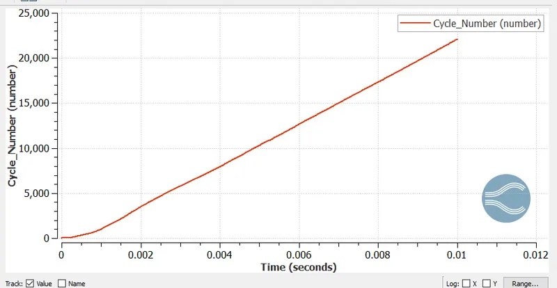
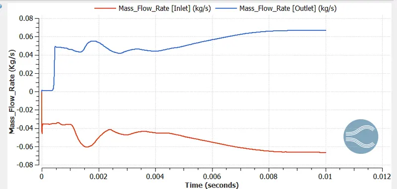
For the simulation time of 0.01 secs and given initial and boundary conditions, the problem runs for around 22500 cycles in 0.01 secs
Mass Flow Rate :
Average Velocity:
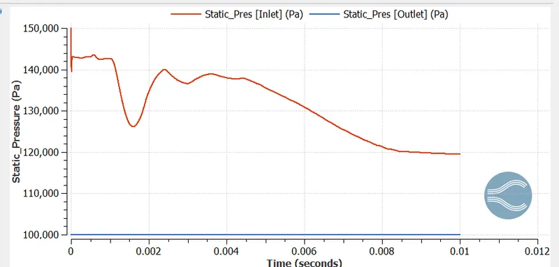
Static Pressure:
Total Pressure:
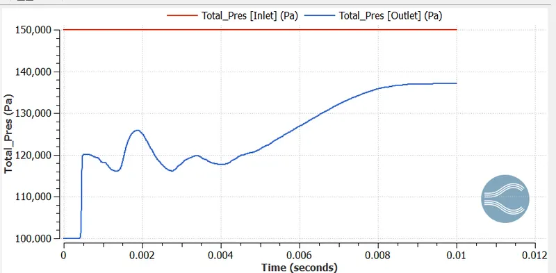
Variation of Pressure:
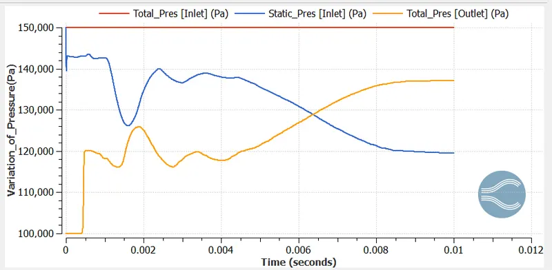
The static pressure decreases at Inlet, total pressure at outlet is due to increase of dynamic pressure at outlet because of ris ein velocity past Throttle.
Number of Total Cells through the entire simulation:
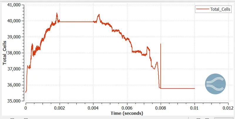
Thee number of cells in the domain can be seen varying throughtout the simulation. Since throttle rotates during simulation, in the cross section view, the area can be seen changing continuosly. So due to change in area of throttle, the cell number increases for first 2 m.seconds at throttle as finer mesh is produced there due to applied Fixed embedding. Since it maintains the same position for next 2 m.seconds cell number remains constant in domain and cell number is around 40000. and for next 4 ms it comes back to original position with initial nuber of cell count of 35800.
Orientation of flow / Visualisation of Velocity vector:
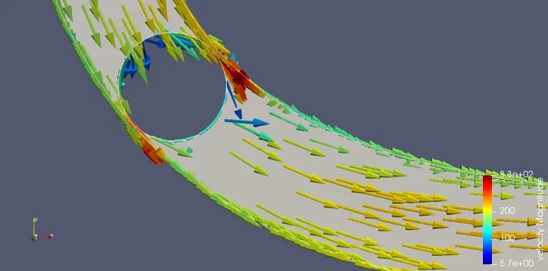
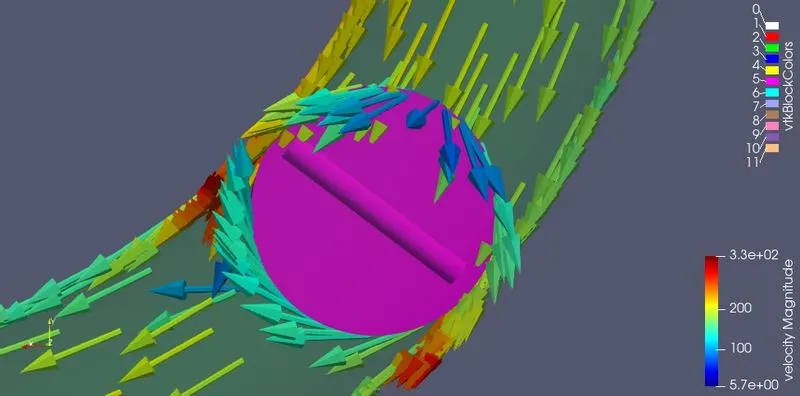
The fashion in which the fluid flows inside the elbow can be with the help of vectors which are oriented in the direction of fluid flow. There are more vectors near the throttle indicating the increased flow rate and velocity. Some of the vectors can be seen directing above the throttle.
Streamline Flow inside the Elbow geometry:
Streamlines near the Throttle:
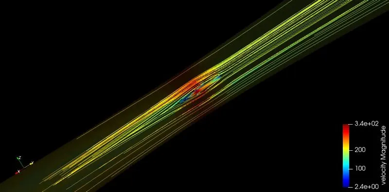
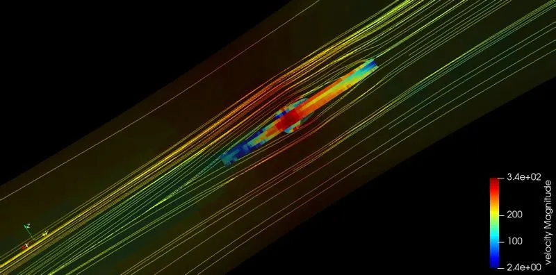
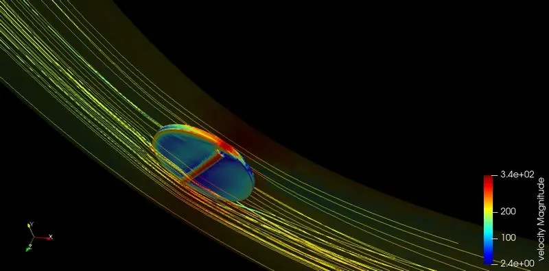
The steamlines indicates the velocity flow in the elbow. At throttle, streamlines clearly indicates the flow velocity on its 4 sides. Velocity is maximum in the consticted region due to reduced area and can be seen in red color. Past the throttle velocity increases and flows towards outlet at higher velocity.
Animation of Steamline flow on Throttle:
The rotation of the throttle can be seen clearly and the flow of the fluid around it for complete simulation time can be seen in animation. The velocity also increases near throttle and can be seen in the color variation of streamlines and on the throttle.
Conclusion:
Studied the effect on flow variables due to the presence of the throttle inside the body.
Increase of static pressure at throttle due to flow termination along with reduction in velocity is analysed.
In the wake region, the flow rate reduces and it results in reduction of both pressure and velocity of flow.
In the constricted region near throttle, velocity reaches its maximum due to reduced area and it results in increase of dynamic pressure too. Velocity increases past the throttle and maximum velocity is around 330m/s.
Better results are captured with more of number of cells near throttle which are created using fixed embedding. More number of cells, finer the mesh, better the results and higher the simulation time.
Transient simulation carried out to rotate the throttle inside the body to vary the rate of flow and studied variation of flow variables on throttle and past the throttle.
Transient simulation takes much more number of cycles for simulation and simulation time is way higher than the steady state simulation.