Week 9 - Mini project - Flow over an Airfoil
Aim:
To Simulate flow over a 4 digit NACA 2412 Airfoil for Angle of Attacks = 1º, 5º, 10º, 15º
and to calculate Drag co-efficient Vs Angle of Attack, Lift co-efficient vs Angle of Attack and Compare the effect of turbulence models on the above two results for the inlet Reynolds number is 2,00,000.
Theory:
An airfoil is the cross-sectional shape of a wing, blade of a propeller rotor or turbine or sail. The lift on an airfoil is primarily the result of its angle of attack. When oriented at a suitable angle, the airfoil deflects the oncoming air , resulting in a force on the airfoil in the direction opposite to the deflection. This force is known as aerodynamic force and can be resolved into two components: lift and drag. Most foil shapes require a positive angle of attack to generate lift, but cambered airfoils can generate lift at zero angle of attack. This turning of the air in the vicinity of the airfoil creates curved streamlines, resulting in lower pressure on one side and higher pressure on the other. This pressure difference is accompanied by a velocity difference, via Bernoulli's principle, so the resulting flow field about the airfoil has a higher average velocity on the upper surface than on the lower surface. In some situations the lift force can be related directly to the average top/bottom velocity.
An airfoil is a streamlined shape that is capable of generating significantly more lift than drag. Airfoils are highly-efficient lifting shapes, able to generate more lift than similarly sized flat plates of the same area, and able to generate lift with significantly less drag.Subsonic flight airfoils have a characteristic shape with a rounded leading edge, followed by a sharp trailing edge, often with a symmetric curvature of upper and lower surfaces and these are called Symmetric Airfoils. Airfoils have potential for use in the design of aircraft, propellers, rotor blades, wind turbines and other applications of aeronautical engineering.
A solid body moving through a fluid produces an aerodynamic force. The component of this force perpendicular to the relative freestream velocity is called Lift.
The equation for Lift,L is given by `L = (1/2 * rho * V^(2)* S * Cl)`
The component parallel to the relative freestream velocity is called Drag.
The equation for Drag, D is given by `D = (1/2 * rho * V^(2)* S * Cd)`
where `rho` is density of fluid which Airfoil is encountering, S is the Area of the airfoil, V is the velocity, Cl and Cd are coefficeint of Lift anf Coeffiecint of drag.
Nomenclature of Airfoil:
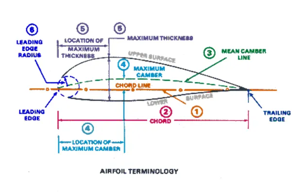
The leading edge is the point at the front of the airfoil that has maximum curvature (minimum radius).
The trailing edge is defined similarly as the point of maximum curvature at the rear of the airfoil.
The chord line is the straight line connecting leading and trailing edges.
The chord length, or chord, is the length of the chord line. That is the reference dimension of the airfoil section.
The mean camber line or mean line is the locus of points midway between the upper and lower surfaces. Its shape depends on the thickness distribution along the chord.
The suction surface (upper surface) is generally associated with higher velocity and lower static pressure.The pressure surface (lower surface) has a comparatively higher static pressure than the suction surface. The pressure gradient between these two surfaces contributes to the lift force generated for a given airfoil.\
Some important parameters to describe an airfoil's shape are its camber and Thickness.
Camber is the maximum perpendicular distance between the mean camber line and the chord line.
The thickness of an airfoil varies along the chord. It may be measured in either of two ways:
Thickness measured perpendicular to the camber line.
Thickness measured perpendicular to the chord line.
An airfoil of the NACA 4-digit series such as the NACA 2412 (to be read as 2 – 4 – 12) describes an airfoil with a camber of 0.02 chord located at 0.40 chord, with 0.12 chord of maximum thickness.
Angle of Attack:
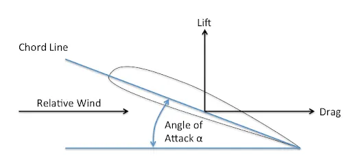
The Angle of Attack is the angle at which relative wind meets an Airfoil. It is the angle formed by the Chord of the aerofoil and the direction of the relative wind or the vector representing the relative motion between the aircraft and the atmosphere. The lift on an airfoil is primarily the result of its angle of attack. Different angle of attack produces different value of lift and drag. Increasing angle of attack is associated with increasing lift coefficient up to the maximum lift coefficient, after which lift coefficient decreases The angle of attack at which more lift and less drag are produced is the most suitable AOA. The critical angle of attack is the angle of attack which produces the maximum lift coefficient. This is also called the Stall angle of attack.
Simulation Process:
Geometry Preparation
Import all the coordinate points of the NACA 2412 Airfoil to Solidworks CADD software and attach them and make a 3D model. Then save th efile in the STL format so that it can be compatible with COnverge Studio.
Import the file of geometry of the NACA aifoil in STL extension into Converge.
Transform the scale of the aifoil to 0.1 so that the chord length of airfoil will be 0.1m. Rotate the airfoil to the required angle of attack.
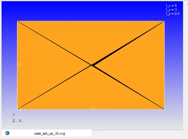
Now the virtual wind tunnel needs to be created. The length of it should be 50 times chord length and height should be 30 times. So go to Create > Vertex and create 4 vertices with coordinates (2.5, 1.5), (2.5, -1.5), (-2.5, 1.5) and (-2.5, -1.5) so that the length and height of the wind tunnel would be 5m and 3m respectively.
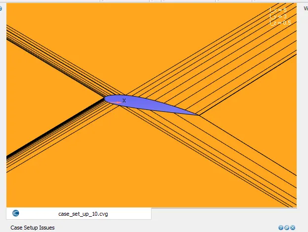
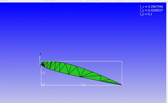
go to repair, Patch these vertex with one end of the airfoil. Delete the remainng part of the airfoil. Copy the entire traingles and offset at 0.5m along z-axis. Loft these set of traingles. Run diagnosis, and if there are any Normal orientations error, go to Transform > Normal, select any triangle >Apply. Now if there are no errors in the model, our airfoil with virtual wind tunnel will be ready for simulation and looks like below for angle of attack = 10 Degrees
Now go to boundary > Flag and select create multiple boundaries.
Geometry clean up and Boundary Flagging:
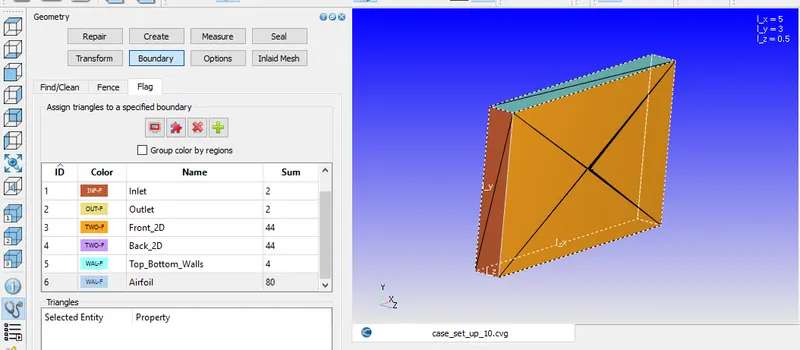
Above figure shows the geometry of the aifoil inside virtual wind tunnel. Geometry is flagged into inlet, outlet, Top_Bottom_wall, Front_2D, Back_2D and the Airfoil. Flow over the airfoil for different angle of attacks is visualised and values of coefficents of lift and drag for these angle of attacks(AOA) are calculated.
Dimensions of Geometry:
Lx = 5m
Ly = 3m
Lz = 0.5m
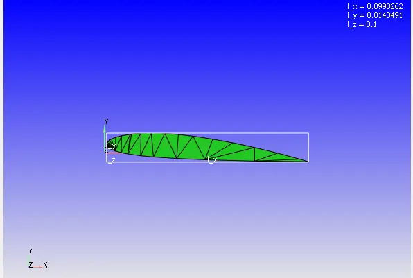
Chord length of Airfoil = 0.1m
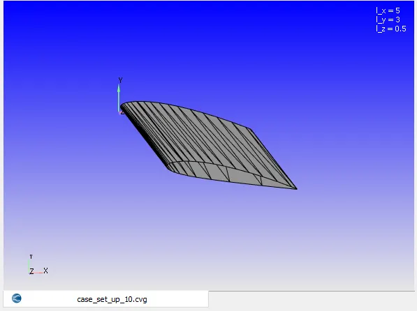
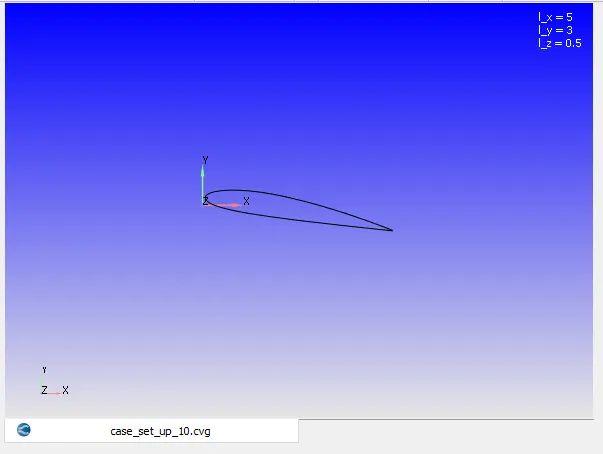
Visualisation of Aifoil :
Case Setup:
1. Applications type: Time - Based
2. Materials:
Select default values for Gas Simulation and Global Transport Properties and Select Air as Predefined Mixture
Species : Add N2 and O2 in Gas
as Air is the working fluid
3.Initial Condition and Events:
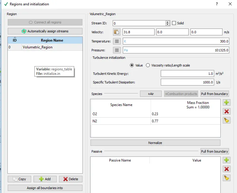
Add a region as Volumetric_Region in regions and Initialisation and intialise species value with below mass fraction
O2 - 0.23
N2 - 0.77 whose combination makes the Air as the working fluid for simulation.
Since the Inlet Reynolds number is 2,00,000. We have `Re = (rho * V * L)/(mu)`
So `V = (R * mu)/(rho* L)`
where R is reynolds number and is R = 2,00,000
`mu` is dynamic viscosity of Air and `mu` = 1.846 * `10^(-5)` kg/m s at 300 K
`rho` is density of air and `rho` = 1.161 `(kg)/m^3` at 300 K
L is the chord length of airfoil and is 0.1 m. Subsituting all these gives
V = `(200000** 1.846 **10^(-5))/(1.161**0.1)` = 31.8 m/s
So initialise the Velocity to 31.8 m/s along X-axis at Inlet with 300 K temperature and 1 atm Pressure.
4. Boundary Conditions:
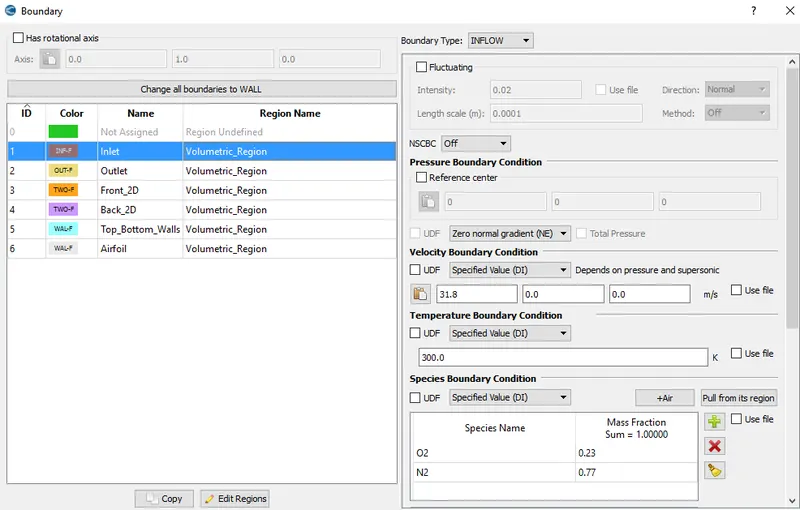
Inlet
Boundary type - INFLOW.
Pressure - Zero Normal Gradient (Neumann BC)
Velocity - 31.8 m/s along x-axis --- Same value as of regions and Initialisation
Temperature - 300 K
Species - N2 = 0.77 and O2 = 0.23
Outlet
Boundary type - OUTFLOW.
Pressure - Zero Normal Gradient (Neumann BC)
Velocity - Zero Normal Gradient (Neumann BC)
Temperature - 300 K
Species - N2 = 0.77 and O2 = 0.23
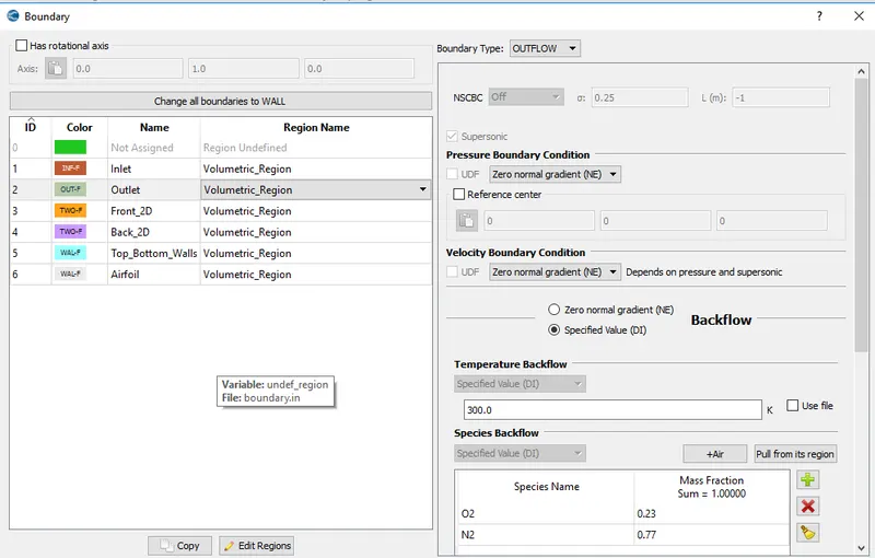
Also mention O2 and N2 species dor Backflow ( if it occurs due to adverse pressure)
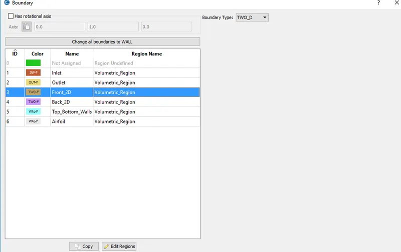
Front and Back Boundaries
Make thes eboundaries as 2D since the simulation is Two Dimensional
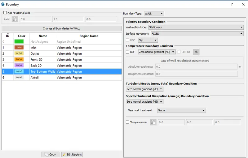
Top and Bottom Walls:
Select boundary type as WALL with Stationary wall motion type.
Provide Slip Velocity BC
Airfoil:
Select boundary type as WALL with Stationary wall motion type.
Provide Law of Wall for Velocity and Temperature BC
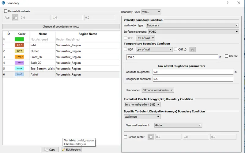
Select Volumetric_Region as Region name for all the boundaries since Volumetric_Region is the region created for the boundaries.
- Simulation Parameters:
Run parameters:
Solver : Transient
Simulation mode: Full hydrodynamic
Turn off use shared memory.
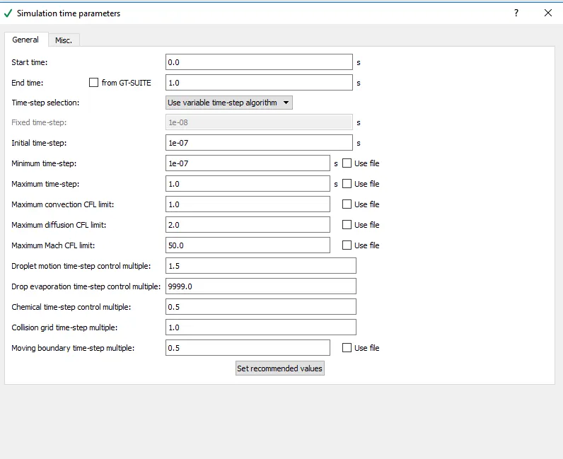
Simulation Time Parameters:
Start time - 0 seconds
Calculating end time for Simulation:
Velocity at the Inlet is 31.8 m/s .
The Length of the Virtual Wind Tunnel is Lx = 5m. So keeping these values, time needed for the fluid to flow from inlet to outlet will be
`Speed = (distance )/ (time)`
so `time = (distance) / (speed)`
time = 5m / (31.8m/s) = 0.157 seconds
and this time is called as Flow Through Time and here it is around 0.1572 seconds.
Simulation is ran for around 6 times of this flow through time to capture all required values over the Airfoil. So
End time = 6 * Flow through time = 6* 0.1572 = 0.9433 seconds and thus it is approximated to 1 seconds.
End time - 1 seconds
Intial time step : 1e-7 s
Minimum time step:1e-7 s
Maximum Time step: 1 s
Maximum convection CFL limit: 1
Leave the rest as Default values.
And the same is shown in below figure
Solver Parameters:
N-S solver Scheme - PISO
N-S Solver Type - Density Based
- Physical Models:
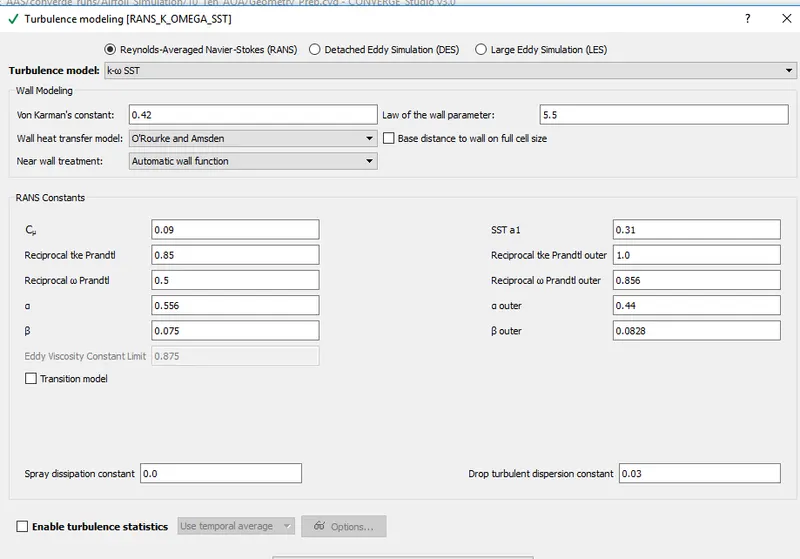
Turbulence model : RNG k -`epsilon` in RANS and K-`omega` SST in RANS and these two models are compared and the best model is selected
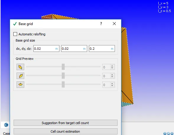
- Grid Control :
Base grid : dx=0.02m dy= 0.02m and dx = 0.2 m
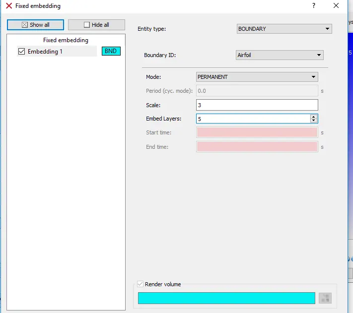
Add fixed Embedding in Grid control
Fixed Embedding:
`Embedded Mesh size = (base mesh size) / (2^(SCALE)`
Over the Airfoil major changes in the flow variables occur. In Order to capture the results accurately over the Airfoil for different AOAS , fine mesh will be need with more cells. Making the mesh size smaller in the entire domain is unnecessary as it would increase the simulation time by very large amount. So mesh size is reduced at the Airfoil alone with the help of a technique called Fixed Embedding. Fixed Embedding of Scale of 3 makes the reduces the base mesh size by 8(2^3) times and embedded layers 5 means the mesh size is further reduced by 8 times at the Airfoil boundary with 5 layers. So fixed embedding is provided at the Airfoil boundary with Embed layers being 5 and scale of 3 using the PERMANENT mode.
- Output/Post-processing
In post variable selection, under Species tab, add N2 and O2 in mass fraction box.
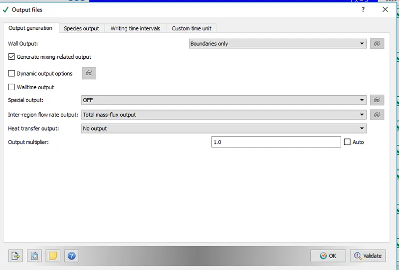
In the Output generation tab under Output files, select Boundaries only for Wall Output as this will dump wall averaged output data which is very much important for any external aerodynamic simulations.
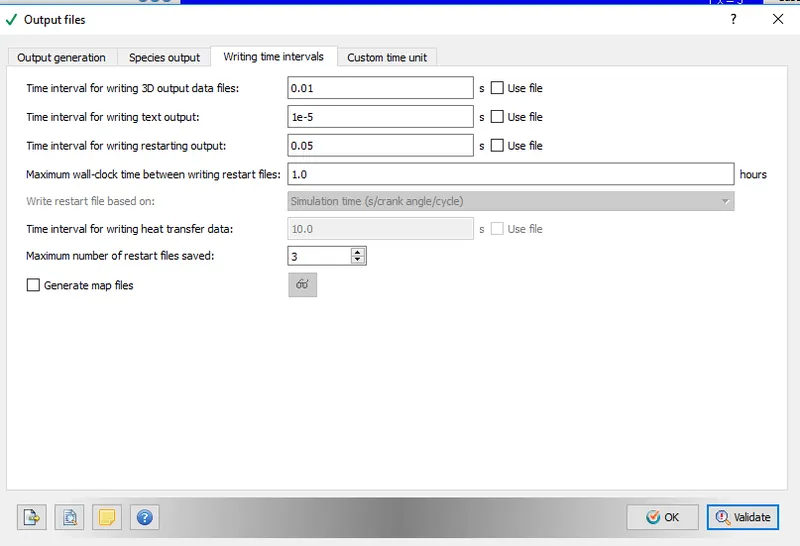
In output files, under Writing time intervals tab, in order to obtain 100 3D output files to cpature the results accurately, time interval for writing 3D output data files and restarting files is specified as 0.01 sec and 0.05 sec since the end time is 1 seconds. 1e-5 sec is provided to time interval for writing text output so outputs are obtained at each cycle of simulation.
Now Export All these input files to a directory. Open CYGWIN, navigate to the directory where all these folders are saved and run the following command ;
mpiexec.exe -n 4 converge.exe restricted </dev/null> logfile_006 &
which runs the simulation with 4 processors using converge executable and outputs are dumped into a file called logfile_006 with job being ran in backend.
Outputs/Post -Processing:
Post processing is performed in the paraview software using the group files with ..vtm extension created in the post processor of Converge
Case-1 : Angle of Attack = 1º
Geometry:
Mesh:
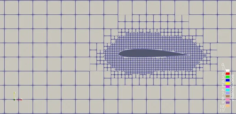
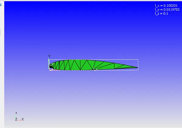
We ca see the refinement in the mesh size around the airfoil. The size of the mesh around airfoil is reduced by 8 times that of the base mesh and this refinement is due to the provided fixed embedding technique to capture accurate results possible over the airfoil.
Pressure Contour:
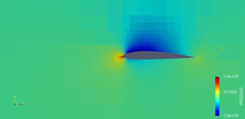
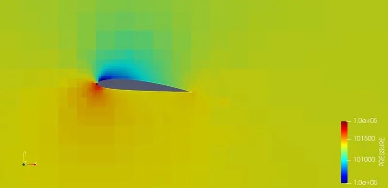
Pressure is lower on the top surface of airfoill than the bottom surface. This difference in pressure over the surfaces or the pressure gradient is the reason behind the production of lift. We can also see the stagnation point in front of the leading edge of the airfoil. The stagnation point is the point where flow comes to rest and the static pressure is higher at this stagation point and the same can be seen in the contour. The pressure difference between stagnation point and trailing edge draws the flow from leading edge to trailing edge over the uper and lower surface.
Velocity Contour:
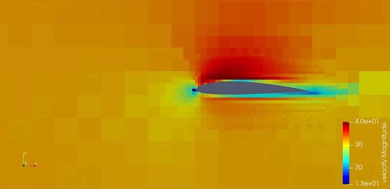
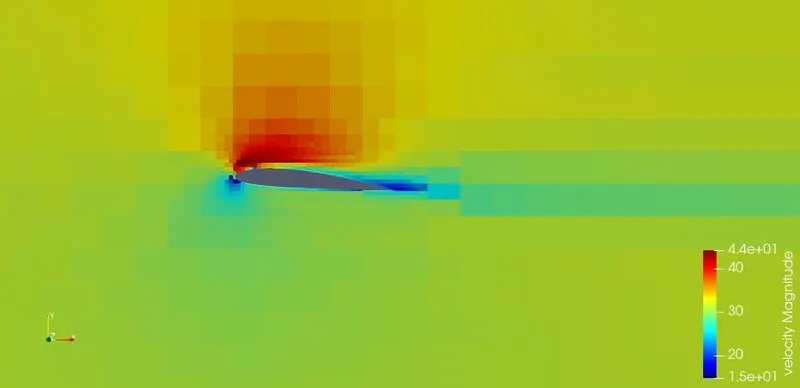
The higher the velocity, lower the pressure. Since the velocity is higher on the upper surface of the airfoil it leads to lower pressure and thus making a pressure difference between surfaces and leads to th eproduction of lifty. We can also see the velocity being minimum on the leading edge of airfoil. This is the region where flow almost comes to rest leading to reduced velocity and increased pressure and this region is called stagnation point.
Orientation of Velocity Vectors:
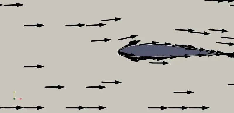
We can see the flow remains attached to the airfoil on both upper and lower surfaces and also their is not much recirculation zones created
Pressure Force along X-axis:
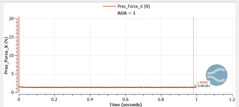
These values are retrived from the folder Wall output - boundaries only - folders which have the average values of the output data around the selected boundary. IN this case we have selected the airfoil boundary so we have th eaverage values of the flow variables around airfoil.
The Average Pressure force along X-axis is nothing but the drag force as The component parallel to the relative freestream velocity is called Drag. Here the value is 1.4N. So drag coeffeiceint can be calculated from equation for Drag, D which is given by `D = (1/2 * rho * V^(2)* S * Cd)`
So coeffiecient if Drag, `Cd =(2 * D)/(rho * V^(2)*S)`
where D = 1.4N
rho = 1.225 kg/m3 is density of Air
V = 31.8 m/s is the freestream velocity flowing from the inlet
S = 0.1 is the chord length (in this case) - Normally it would be area.
So `Cd = (2 ** 1.4)/(1.225 **31.8^(2)**0.1)`
Cd = 0.0226 for angle of Attack = 1º
Pressure force along Y-axis:
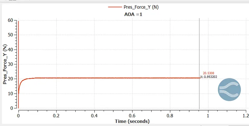
The Average Pressure force along Y-axis is nothing but the lift forceas The component of this force perpendicular to the relative freestream velocity is called Lift. The equation for Lift,L is given by `L = (1/2 * rho * V^(2)* S * Cl)`
So coeffiecient of Lift, `Cl =(2 * L)/(rho * V^(2)*S)`
where L = 20.5 N
So `Cl = (2 ** 20.5)/(1.225 **31.8^(2)**0.1)`
Cl = 0.3309 for Angle of Attack = 1º.
Case-2.1: Angle of Attack = 5º
Turbulence Model - K-`omega` SST
Geometry:
Mesh:
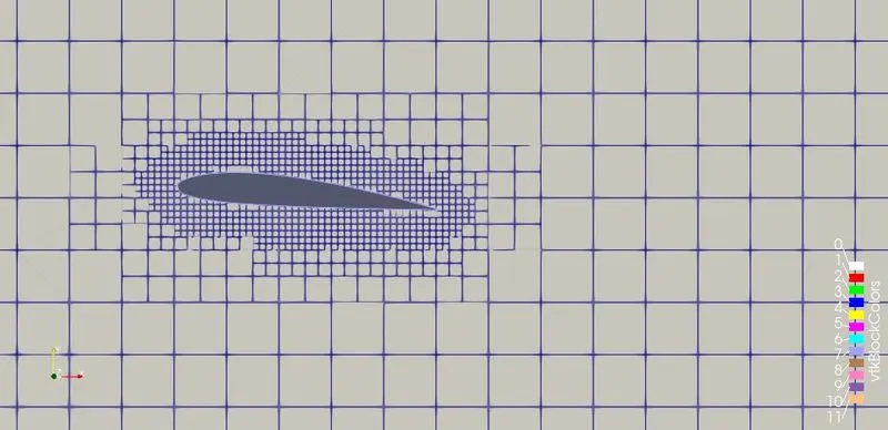
We ca see the refinement in the mesh size around the airfoil. The size of the mesh around airfoil is reduced by 8 times that of the base mesh and this refinement is due to the provided fixed embedding technique to capture accurate results possible over the airfoil.
Pressure Contour:
Velocity Contour:
Orientation of Velocity Vectors:
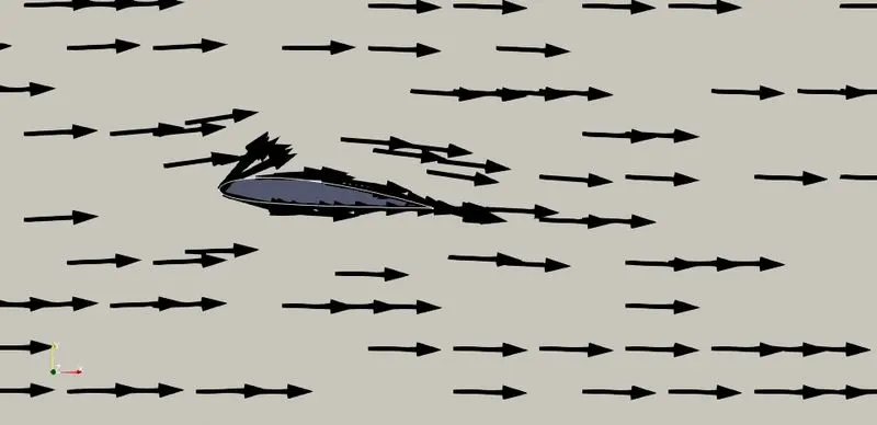
We can see some of the vectors moving away from the leading edge. The flow reattaches at the trailing edge upon passing through upper and lower surfaces and also flows smoothly on surfaces and remains attached to them. Also their is not much recirculation zones created
Pressure Force along X-axis:
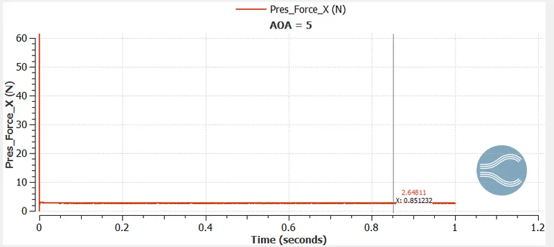
The Average Pressure force along X-axis is nothing but the drag force as The component parallel to the relative freestream velocity is called Drag. Here the value is 2.64N. So drag coeffeiceint can be calculated from equation for Drag, D which is given by `D = (1/2 * rho * V^(2)* S * Cd)`
So coeffiecient if Drag, `Cd =(2 * D)/(rho * V^(2)*S)`
where D = 2.64N
rho = 1.225 kg/m3 is density of Air
V = 31.8 m/s is the freestream velocity flowing from the inlet
S = 0.1 is the chord length (in this case) - Normally it would be area.
So `Cd = (2 ** 2.64)/(1.225 **31.8^(2)**0.1)`
Cd = 0.0462 for angle of Attack = 5º
Pressure force along Y-axis:
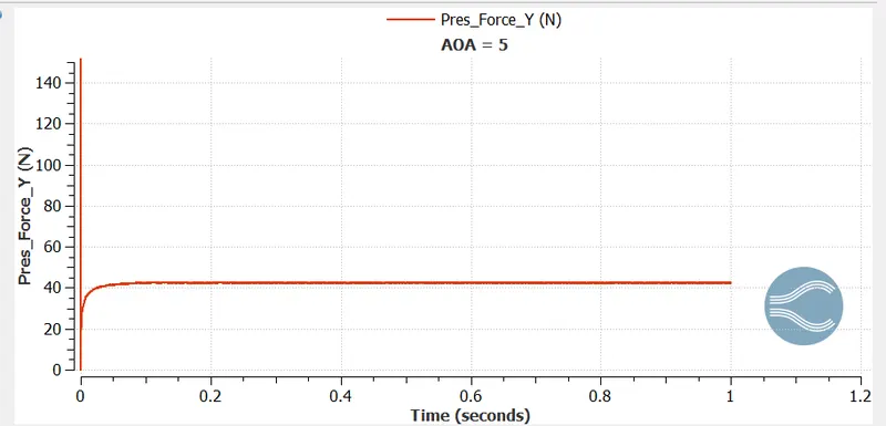
The Average Pressure force along Y-axis is nothing but the lift forceas The component of this force perpendicular to the relative freestream velocity is called Lift. The equation for Lift,L is given by `L = (1/2 * rho * V^(2)* S * Cl)`
So coeffiecient of Lift, `Cl =(2 * L)/(rho * V^(2)*S)`
where L = 41 N
So `Cl = (2 ** 41)/(1.225 **31.8^(2)**0.1)`
Cl = 0.66195 for Angle of Attack = 5º.
Case-2.2: Angle of Attack = 5º
Choosing the Correct Model for Current external Aerodynamic Simulation.
Turbulence Model - RNG K -`epsilon`
Since our aim in the current simulation is to accurately predict the boundary layer velocity , because the developing boundary layer will tend to separate near airfoil( due to a changing pressure gradient and not because of sharp edges or discontinuities in the geometry as in case of Prandtl Meyer Shock Ananlysis Problem) , using low-Re model is recommended.
Low-Re models are also required for accurate pressure-drop or drag calculations. It is highly recommend to use the Shear Stress Transport (SST) model, although all ω-based models or ε-based models with enhanced wall treatment may be used.
For flows where wall-bounded effects are not a priority, or if separation is expected to occur only due to sharp changes in the geometry, an ε-based wall function approach is more than sufficient.
All ω-based models and the SST model are capable of resorting to a wall function formulation (automatic wall treatment) in the presence of coarse mesh resolutions near the wall.
Also when RNG - k `epsilon` model is used, for 5º angle of attck, time taken for simulation is aroud 8500 seconds and the time for K-`omega` SST is 6300 seconds and results are quite accurate near airfoil when Low Re Model K`omega` SST is used.
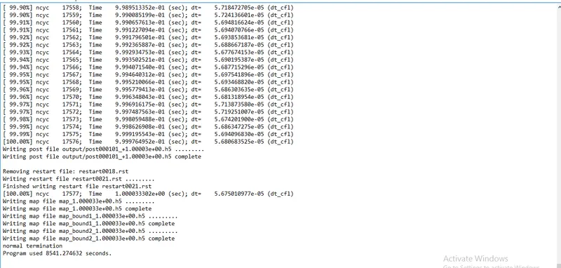
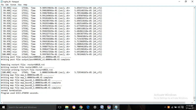
Since for our current simulation, there is large variation of pressure gradient near airfoil, there is formation of voundary layer and seperation of flow near airfoil, K-`omega`SST model is used for all cases in order accurately predict boundary layer velocity. Because of these reasons K-`omega`SST model is used as turbulence model for all angle of attacks.
Animations:
Pressure Contour:
Velocity Contour:
Case -3 : Angle of Attack = 10º
Geometry:
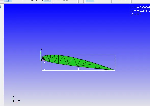
Mesh:
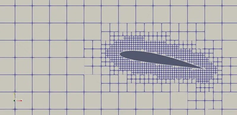
We can see the refinement in the mesh size around the airfoil. The size of the mesh around airfoil is reduced by 8 times that of the base mesh and this refinement is due to the provided fixed embedding technique to capture accurate results possible over the airfoil.
Pressure Contour:
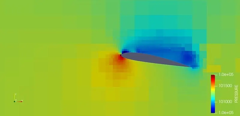
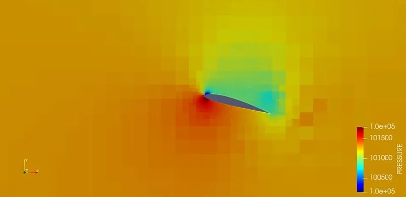
We can see the lower pressure on the entire upper surface of the airfoil and this regin of low pressure is much larger than previous cases. So this creates larger pressure gradients between upper and lower surfaces and this increases the lift. It is also involved with some disadvantage by the fact that tis low pressure creates backflow and recirculation.
Velocity Contour:
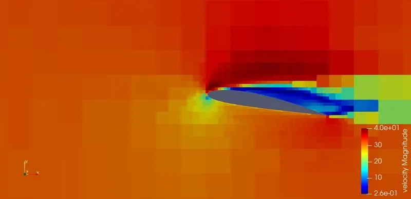
Orientation of Velocity Vectors:
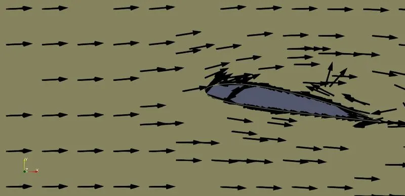
We can see the flow remains attached to the airfoil on both upper and lower surfaces . Also their is a backflow from trailing edge to leading edge due to adverse pressure gradient. At some point the pressure on top surface of airfoil is soo less that flow starts to reverse and this creates some recirculation zones and can be seen on top surface of airfoil and above trailing edge and this increases the drag.
Pressure Force along X-axis:
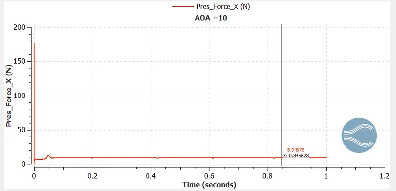
The Average Pressure force along X-axis is nothing but the drag force as The component parallel to the relative freestream velocity is called Drag. Here the value is 8.9N. So drag coeffeiceint can be calculated from equation for Drag, D which is given by `D = (1/2 * rho * V^(2)* S * Cd)`
So coeffiecient of Drag, `Cd =(2 * D)/(rho * V^(2)*S)`
where D = 8.9N
rho = 1.225 kg/m3 is density of Air
V = 31.8 m/s is the freestream velocity flowing from the inlet
S = 0.1 is the chord length (in this case) - Normally it would be area.
So `Cd = (2 ** 8.9)/(1.225 **31.8^(2)**0.1)`
Cd = 0.143 for angle of Attack = 10º
Pressure force along Y-axis:
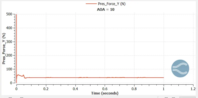
The Average Pressure force along Y-axis is nothing but the lift forceas The component of this force perpendicular to the relative freestream velocity is called Lift. The equation for Lift,L is given by `L = (1/2 * rho * V^(2)* S * Cl)`
So coeffiecient of Lift, `Cl =(2 * L)/(rho * V^(2)*S)`
where L = 56 N
So `Cl = (2 ** 56)/(1.225 **31.8^(2)**0.1)`
Cl = 0.9041 for Angle of Attack = 10º.
Case -4 : Angle of Attack = 15º
Geometry:
Mesh:
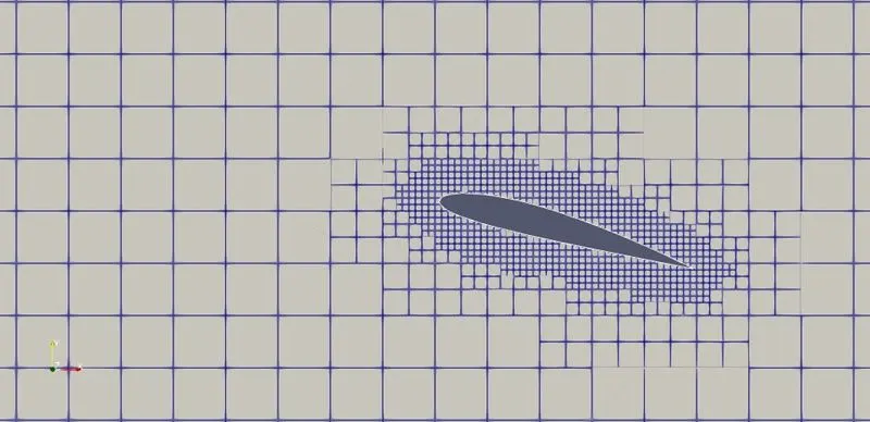
We can see the refinement in the mesh size around the airfoil. The size of the mesh around airfoil is reduced by 8 times that of the base mesh and this refinement is due to the provided fixed embedding technique to capture accurate results possible over the airfoil.
Pressure Contour:
Velocity Contour:
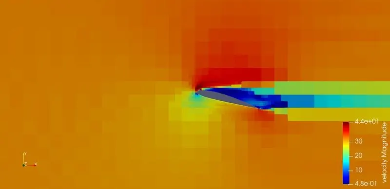
Orientation of Velocity Vectors:
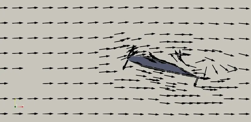
We can see the flow doesnt remains attached to the airfoil on both upper and lower surfaces . Also their is a backflow from trailing edge to leading edge due to adverse pressure gradient. At some point the pressure on top surface of airfoil is soo less that flow starts to reverse and this creates some recirculation zones and can be seen on top surface of airfoil and above trailing edge and this increases the drag. The recirculation zone can be seen clearly at the back of the trailing edge and this increases the drag by huge amount.
So 15º AOA might be above the Critical angle of attack or stalling angle of attack which means it shouldnt be operate at this angle beacuse itll lead to increased drag with reduced lift.
Pressure Force along X-axis:
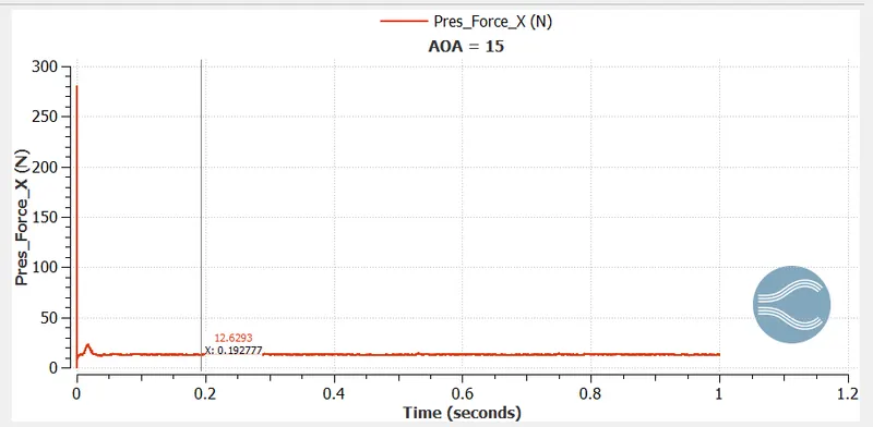
The Average Pressure force along X-axis is nothing but the drag force as The component parallel to the relative freestream velocity is called Drag. Here the value is 12.6N. So drag coeffeiceint can be calculated from equation for Drag, D which is given by `D = (1/2 * rho * V^(2)* S * Cd)`
So coeffiecient if Drag, `Cd =(2 * D)/(rho * V^(2)*S)`
where D = 12.6N
rho = 1.225 kg/m3 is density of Air
V = 31.8 m/s is the freestream velocity flowing from the inlet
S = 0.1 is the chord length (in this case) - Normally it would be area.
So `Cd = (2 ** 12.6)/(1.225 **31.8^(2)**0.1)`
Cd =0.2034 for angle of Attack = 15º
Pressure force along Y-axis:
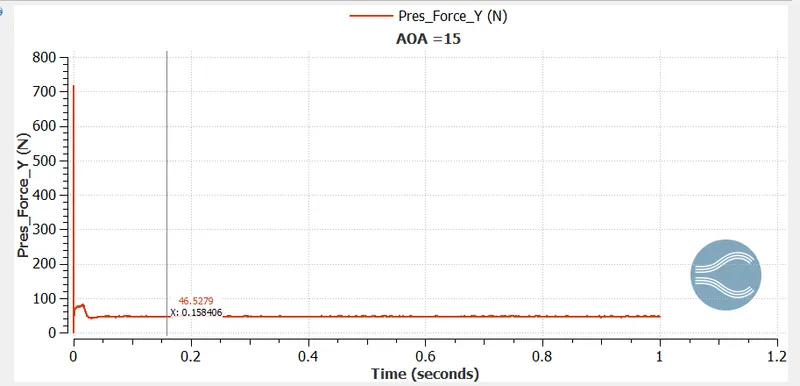
The Average Pressure force along Y-axis is nothing but the lift forceas The component of this force perpendicular to the relative freestream velocity is called Lift. The equation for Lift,L is given by `L = (1/2 * rho * V^(2)* S * Cl)`
So coeffiecient of Lift, `Cl =(2 * L)/(rho * V^(2)*S)`
where L =46.5 N
So `Cl = (2 ** 46.5)/(1.225 **31.8^(2)**0.1)`
Cl =0.7507 for Angle of Attack = 15º
Conclusion:
Cl and Cd V/s Angle of Attack:
| Angle of Attack | Coefficient of Lift (Cl) | Coefficient of Drag (Cd) |
| 1º | 0.33097 | 0.022603 |
| 5º | 0.66195 | 0.042623 |
| 10º | 0.90412 | 0.143691 |
| 15º | 0.75075 | 0.203428 |
Plot of Cl v/s Angle of Attack:
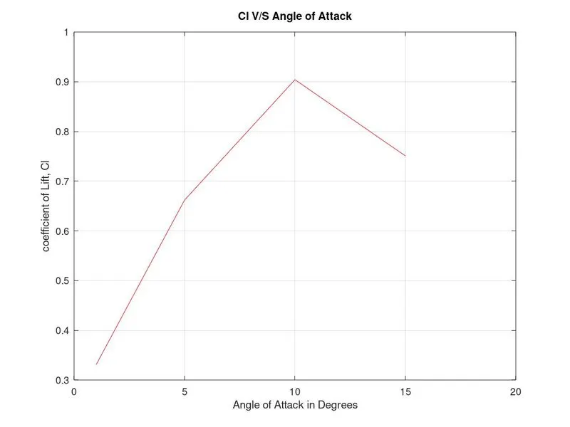
We can see the increase in the coefficeint of lift and lift with the increase in the angle of attck until a some value of AOA(Here 10). With further increase after this, the angle 15º is above the critical angle of attack, due to the adverse pressure gradient flow starts to reverse and flows from trailing edge to leading edge on the upper surface and this creates recirculation zone. This leads to the decreases lift above crictical angle or popularly known as stalling angle.
Plot of Cd v/s Angle of Attack:
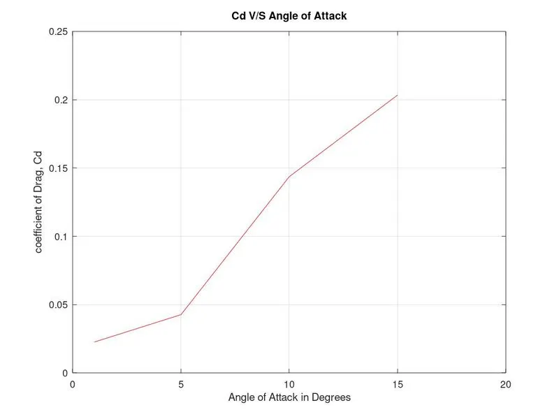
We can see the increase in the coefficeint of drag and ldrag with the increase in the angle of attack. For any angle above critical angle of attack, due to the adverse pressure gradient flow starts to reverse and flows from trailing edge to leading edge on the upper surface and this creates recirculation zone. This leads to increase in the drag coefficeint by large amount above crictical angle. Cd value is quite higher in all AOAs because of lesser considered value for S.
- Successfully studied the effect of turbulence models in producing results and k-omega SST produces results that are quite near to the experimental results. So this turbulence model is selected for the simulation.
- Succesfully simulated flow over airfoil for different angle of attacks and variation of flow properties over airfoil are studied.
The critical angle of attack is the angle of attack which produces the maximum lift coefficient. This is also called the Stall angle of attack. From our si,ulation result we can say that this stall angle of attck is in between 10º and 15º
Below the critical angle of attack, as the angle of attack decreases, the lift coefficient decreases. Above the critical angle of attack, as the angle of attack increases, the air begins to flow less smoothly over the upper surface of the airfoil and begins to separate from the upper surface.
As the angle of attack increases, the upper surface separation point of the flow moves from the trailing edge towards the leading edge. At the critical angle of attack, upper surface flow is more separated and the airfoil or wing is producing its maximum lift coefficient. As the angle of attack increases further, the upper surface flow becomes more fully separated and the lift coefficient reduces further. So the airfoil should not be operated above stall angle of attack as it would prdouce more drag with reduced lift coefficeint.