Week 5.1 - Mid term project - Solving the steady and unsteady 2D heat conduction problem
Aim:
To solve Steady and Unsteady 2D heat conduction equation by implementing various iterative techniques in MATLAB.
Theory:
Heat conduction is the process of transmission of heat energy from one particle of the medium to the other but here each particle of the medium stays at its own position.
In this condition, we are considering the conduction is taking place along 2 axes. So it is called 2D heat conduction.
This system can be solved by partial differential equations. It is given by
`(dT)/dt + alpha((d^(2)T)/dx^2 + (d^(2)T)/dy^2 + (d^(2)T)/dz^2 ) = 0`
The above is 3D transient heat conduction equation. If there is no source term in RHS it is equal to 0. It has time derivative dT/dt
In 2D, the equation is given by
`(dT)/dt + alpha((d^(2)T)/dx^2 +( d^(2)T)/dy^2 ) = 0`
Where alpha is the heat diffusivity term.
The above partial differential equation can be solved using two approaches.
- Steady State Condition
- Transient or Unsteady State Condition
Steady State Conduction
If the temperature at any position remains constant with time and may vary with position, the system is said to be in steady-state.
For a conductor in steady-state, there is no absorption or emission of heat at any cross-section as the temperature at each point remains constant with time.
The partial differential equation in Steady state is given by
`((d^(2)T)/dx^2 + (d^(2)T)/dy^2 ) = 0`
Above equation is elliptic in nature and as it is 2d and involves second order term, central differencing scheme is employed which takes information from all neighboring points.
If Tp is the is the Temperature at the present point of interest then
Tl and Tr are the temperature at left and right point along x-axis and
Tt and Tb are the temperatures at top and bottom point along y-axis.
Transient or Unsteady State Conduction
During transient conduction, the temperatures can change or vary at any part at a given time. This mode of conduction is also termed as “non-steady-state” conduction. The main point that we have to consider here is the object’s time-dependence of temperature.
Non-steady-state conduction usually occurs when a change in temperature is introduced within the outer areas of an object or inside. The temperature change is brought about by the sudden entry of a new source of heat within the object.
The partial differential equation that govern the unsteady state conduction is
`(dT)/dt + alpha((d^(2)T)/dx^2 + (d^(2)T)/dy^2 ) = 0`
The given problem is
Top Boundary = 600 K
Bottom Boundary = 900 K
Left Boundary = 400 K
Right Boundary = 800 K
We need to implement the following methods for solving implicit equations.
- Jacobi
- Gauss-seidel
- Successive over-relaxation
Your absolute error criteria is 1e-4
These partial differential equations can be solved implicitly or explicitly. Explicit method makes use of the values obtained in previous iteration whereas implicit method makes use of the values obtained in the current iteration.
The solution can be solved by 3 Iterative Methods
- Jacobi Iterative Method
- Gauss – Siedal Iterative Method
- Successive Over Relaxation Method
Let’s look at these methods one by one to solve the steady and unsteady 2D heat conduction equation.
Elliptic equation when central scheme is employed can be written as
`((d^(2)T)/dx^2 + (d^(2)T)/dy^2 ) = [(Tl -(2**Tp)+Tr)/(Deltax^2) +( Tt-(2**Tp)+ Tb)/(Deltay^2)]`
Steady State Conduction
Iterative Methods
- Jacobi Method
Here we make use of values that are obtained in the previous iterations to calculate the present iteration values.
Governing equation is
`((d^(2)T)/dx^2 + (d^(2)T)/dy^2 ) = 0`
Simplifying this we will get
`Tp^(n+1) = (1/k) **[(Tl + Tr)/(Deltax^2) +( Tt+ Tb)/(Deltay^2)]^n`
where k is
`k = 2 **((Deltax^2+Deltay^2)/(Deltax^2 * Deltay^2))`
MATLAB Code for Jacobi is
clear all
close all
clc

%Steady State 2D Heat Conduction using Iterative Techniques

%Jacobi Iterative method

%Inputs
%Dimension of Square Domain
L =1 ;

%No of node points along x-axis
nx = 10;

%No of node points along y-axis
ny = nx;

%discretising
x = linspace(0,L,nx);
y = linspace(0,L,ny);

%Calculating step size dx and dy
dx = x(2)-x(1);
dy = y(2)-y(1);

%Initialsing error and defining tolerance
error = 9e9;
tol = 1e-4;  % Tolerance value

%Defining Boundary Conditions
%Value of Temperature at Boundaries in K
T_left = 400;
T_right = 800;
T_top = 600;
T_bottom = 900;

%Initialising Temperature at all nodes inside domain
%Initial Condition - Temperature at all nodes is taken 300K
T = 300*ones(nx,ny);

%providing boundary conditions
T( 1:ny, 1) = T_left;
T( 1:ny, nx) = T_right;
T( 1, 1:nx) = T_top;
T( ny, 1:nx) = T_bottom;

%At corners average temperature value is taken
T(1,1) = (T_left + T_top)/2;
T(1,ny) = (T_right + T_top)/2;
T(nx,1) = (T_bottom+T_left)/2;
T(nx,ny) = (T_bottom + T_right)/2;

%Taking Initial T value to a another Array
T_prev = T;
Told = T;

%Solving Steady State equation
%d^2T/dx^2 + d^2T/dy^2 = 0
% Tp = 1/k *(((Tl + Tr)/2)+((Tb+Tt)/2))
%k = 2((dx^2+dy^2)/(dx^2 * dy^2))

k = 2 * ((dx^2 + dy^2)/(dx^2 * dy^2));

%convergence loop  %Jacobi Method
jacobi_iter = 1;
tic
while (error > tol)                %Convergence loop
    for i = 2:nx-1                 %Spacial loop
        for j= 2:ny-1
            term1 = (Told(i-1,j)+Told(i+1,j))/dx^2;      %left and Right points at older time step
            term2 = (Told(i,j-1)+Told(i,j+1))/dy^2;      %top and bottom points at older time step
            T(i,j) = 1/k *(term1 + term2);
        end
    end
    %Inner term max(abs(T-Told)) is an array and maximum value of that array needs to be taken
    error = max(max(abs(T-Told)));
    Told = T;
    jacobi_iter = jacobi_iter+1;
end
j_steady_time = toc

figure(1)
%Plotting contour of Temperature

contourf(x,y,T,'showtext','on')  %f is used to get filled contour
%Labelling the lines
% clabel(contourf(x,y,T))
colormap(jet)
colorbar
%Reversing the direction of y-axis
set(gca,'ydir','reverse')
xlabel('X-axis')
ylabel('Y-axis')
title_text = sprintf('Method-Steady:Jacobi, Iterations =%d,Time =%d',jacobi_iter,j_steady_time)
title(title_text);
pause(0.03)
Explanation of Code:
The square domain of dimension 1 unit is taken with 10 nodes each along x and y axes.
dx and dy values which are the distance between each nodes is calculated. Error and tolerance values are defined. Error is the difference between the values of present iteration and previous iteration and the iteration process is continued till the error term becomes lesser than the tolerance meaning our system or solution has converged.
Temperature values at the boundaries are defined and at all nodes are initialized and this is called defining initial and boundary conditions.
There is no need to use time values as the temperature remains constant.
Convergence and space loops are initialized and the Jacobi formula is coded. Since it makes use of previous iteration values Told is used which has required previous iteration values.
Error is calculated as the maximum value of difference between the previous and present iteration. Since this will be an array, the maximum value of this array is used as error.
Told values are updated after each iteration and convergence loop is continued till error is greater than tolerance value.
Then the temperature contour is plotted using contour which fills the gap between the lines.
colormap gives the different kind of colors inside the contour. There are various colormaps available like parula, winter, summer, autumn. Jet colormap gives good variation between colors for differentiating the temperature at different regions.
Then y-axis is reversed and time taken for calculation is calculated using tic and toc command.
The same process of coding is used throughout according to the formula of the method used.
Result:
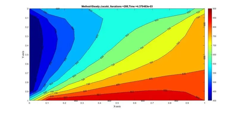
The number of iterations here is 208. So may look to reduce the number of iterations by updating the values in the same iteration.
Gauss – Siedal Method:
Here the value of temperature of the points left and bottom to the present point of the present iteration is used and the temperature value of the right and top points of previous iteration are used to calculate the temperature value of present point for current iteration. That is updated values are used.
`Tp^(n+1) = (1/k) **[(Tl + Tr)/(Deltax^2) +( Tt+ Tb)/(Deltay^2)]^(n+1)`
MATLAB Code for Gauss-Siedal is
clear all
close all
clc

%Steady State 2D Heat Conduction using Iterative Techniques

%Gauss_Siedal Iterative method

%Inputs
%Dimension of Square Domain
L =1 ;

%No of node points along x-axis
nx = 10;

%No of node points along y-axis
ny = nx;

%discretising
x = linspace(0,L,nx);
y = linspace(0,L,ny);

%Calculating step size dx and dy
dx = x(2)-x(1);
dy = y(2)-y(1);

%Initialsing error and defining tolerance
error = 9e9;
tol = 1e-4;  % Tolerance value

%Defining Boundary Conditions
%Value of Temperature at Boundaries in K
T_left = 400;
T_right = 800;
T_top = 600;
T_bottom = 900;

%Initialising Temperature at all nodes inside domain
%Initial Condition - Temperature at all nodes is taken 300K
T = 300*ones(nx,ny);

%providing boundary conditions
T( 1:ny, 1) = T_left;
T( 1:ny, nx) = T_right;
T( 1, 1:nx) = T_top;
T( ny, 1:nx) = T_bottom;

%At corners average temperature value is taken
T(1,1) = (T_left + T_top)/2;
T(1,ny) = (T_right + T_top)/2;
T(nx,1) = (T_bottom+T_left)/2;
T(nx,ny) = (T_bottom + T_right)/2;

%Taking Initial T value to a another Array
T_prev = T;
Told = T;

%Solving Steady State equation
%d^2T/dx^2 + d^2T/dy^2 = 0
% Tp = 1/k *(((Tl + Tr)/2)+((Tb+Tt)/2))
%k = 2((dx^2+dy^2)/(dx^2 * dy^2))

k = 2 * ((dx^2 + dy^2)/(dx^2 * dy^2));

%convergence loop  %Gauss-Siedal Method
gs_iter = 1;
tic
while (error > tol)          %Convergence loop
    for i = 2:nx-1           %Spacial loop
        for j= 2:ny-1
            term1 = (T(i-1,j)+Told(i+1,j))/dx^2;    %left and Right points at new and older time step
            term2 = (T(i,j-1)+Told(i,j+1))/dy^2;    %top and bottom points at new and older time step
            T(i,j) = 1/k *(term1 + term2);
        end
    end
    %Inner term max(abs(T-Told)) is an array and maximum value of that array needs to be taken
    error = max(max(abs(T-Told)));
    Told = T;
    gs_iter = gs_iter+1;
end
gs_steady_time = toc

figure(1)
%Plotting contour of Temperature

contourf(x,y,T,'showtext','on')  %f is used to get filled contour
%Labelling of lines using showtext
colormap(jet)
colorbar
%Reversing the direction of y-axis
set(gca,'ydir','reverse')
xlabel('X-axis')
ylabel('Y-axis')
title_text = sprintf('Method-Steady:G-S, Iterations =%d,Time =%d',gs_iter,gs_steady_time)
title(title_text);
pause(0.03)
Result:
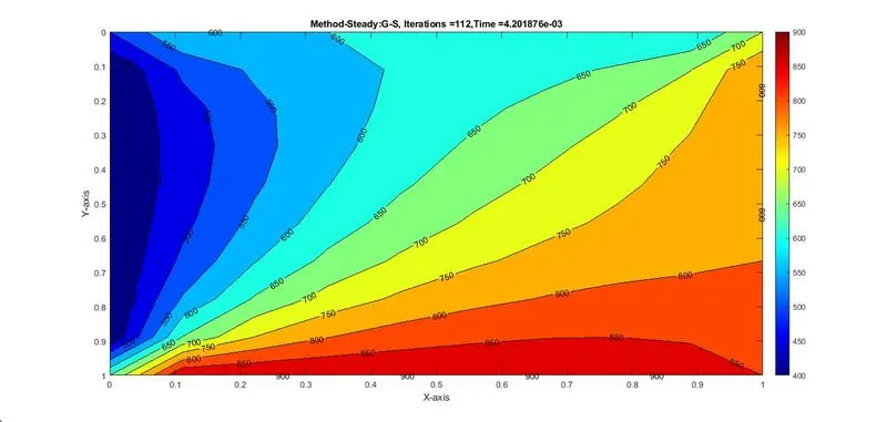
Here number of iterations is 112 which is almost half the number compared to Jacobi. We can reduce the number of iterations just by updating the values in the same iteration.
Successive Over Relaxation Method:
This method is the enhanced iterative solver. It makes use of term called relaxation factor ‘omega’(w) and this value is taken to be 1.2. Either we can use Gauss siedal or Jacobi method here to enhance their performance.
Equation for this method is given by
`Tp^(n+1) = ((1-w)**T^(n)p)+w**((1/k) **[(Tl + Tr)/(Deltax^2) +( Tt+ Tb)/(Deltay^2)]^(n+1))`
MATLAB Code for SOR is
clear all
close all
clc

%Steady State 2D Heat Conduction using Iterative Techniques

%Successive Over Relaxation(SOR) Iterative method

%Inputs
%Dimension of Square Domain
L =1 ;

%No of node points along x-axis
nx = 10;

%No of node points along y-axis
ny = nx;

%discretising
x = linspace(0,L,nx);
y = linspace(0,L,ny);

%Calculating step size dx and dy
dx = x(2)-x(1);
dy = y(2)-y(1);

%Initialsing error and defining tolerance
error = 9e9;
tol = 1e-4;  % Tolerance value

%Defining Boundary Conditions
%Value of Temperature at Boundaries in K
T_left = 400;
T_right = 800;
T_top = 600;
T_bottom = 900;

%Initialising Temperature at all nodes inside domain
%Initial Condition - Temperature at all nodes is taken 300K
T = 300*ones(nx,ny);

%providing boundary conditions
T( 1:ny, 1) = T_left;
T( 1:ny, nx) = T_right;
T( 1, 1:nx) = T_top;
T( ny, 1:nx) = T_bottom;

%At corners average temperature value is taken
T(1,1) = (T_left + T_top)/2;
T(1,ny) = (T_right + T_top)/2;
T(nx,1) = (T_bottom+T_left)/2;
T(nx,ny) = (T_bottom + T_right)/2;

%Taking Initial T value to a another Array
T_prev = T;
Told = T;

%Solving Steady State equation
%d^2T/dx^2 + d^2T/dy^2 = 0
% Tp = 1/k *(((Tl + Tr)/2)+((Tb+Tt)/2))
%k = 2((dx^2+dy^2)/(dx^2 * dy^2))

k = 2 * ((dx^2 + dy^2)/(dx^2 * dy^2));

%convergence loop  %SOR Method
%Defining Relaxation Factor omega w
w = 1.2;
sor_iter = 1;
tic
while (error > tol)           %Convergence loop
    for i = 2:nx-1            %Spacial Loop
        for j= 2:ny-1
            term1 = (T(i-1,j)+Told(i+1,j))/dx^2;           %left and Right points at new and older time step
            term2 = (T(i,j-1)+Told(i,j+1))/dy^2;           %top and bottom points at new and older time step
            T(i,j) = (1-w)*Told(i,j) + w *(1/k *(term1 + term2));
        end
    end
    %Inner term max(abs(T-Told)) is an array and maximum value of that array needs to be taken
    error = max(max(abs(T-Told)));
    Told = T;
    sor_iter = sor_iter+1;
end
sor_steady_time = toc

figure(1)
%Plotting contour of Temperature

contourf(x,y,T,'showtext','on')  %f is used to get filled contour
%Labelling of lines using showtext
colormap(jet)
colorbar
%Reversing the direction of y-axis
set(gca,'ydir','reverse')
xlabel('X-axis')
ylabel('Y-axis')
title_text = sprintf('Method-Steady:SOR, Iterations =%d,Time =%d',sor_iter,sor_steady_time)
title(title_text);
pause(0.03)
Result:
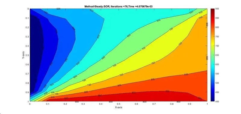
Here number of iterations is 76. So we are reduing the number of iterations by 1/3 times of Jacobi in this method. So it is the enhancer method.
Transient or Unsteady 2D heat conduction:
Here temperatures can change or vary at any part at a given time. We need to make use of time values and the iteration loop need to be continued for atleast 1400 time steps to converge.
The partial differential equation that govern the unsteady state conduction is
`(dT)/dt + alpha((d^(2)T)/dx^2 + (d^(2)T)/dy^2 ) = 0`
We can use explicit method or Implicit method ( Iterative methods) to solve this transient conduction.
Iterative Methods
Jacobi Method
Here values for the previous iterations are used.
Equation is
`Tp^(n+1) = (1/(1+2k1 +2k2)) **[(T^(n)p(prev)+k1**(Tl + Tr)^(n)+k2** (Tt+ Tb)^(n)]`
where k1 and k2 are the CFL values and are given by
`k1= alpha **((Deltat)/(Deltax^2))`
`k2= alpha **((Deltat)/(Deltay^2))`
and summation of this needs to be less than 0.5 for stable solution.
where alpha is the thermal diffusivity term and it is taken as 1.4.
MATLAB Code for Jacobi is
clear all
close all
clc

%Unsteady State 2D Heat Conduction using Iterative Techniques

%Jacobi Iterative method

%Inputs
%Dimension of Square Domain
L =1 ;

%No of node points along x-axis
nx = 10;

%No of node points along y-axis
ny = nx;

%discretising
x = linspace(0,L,nx);
y = linspace(0,L,ny);

%Calculating step size dx and dy
dx = x(2)-x(1);
dy = y(2)-y(1);

%Time values
dt = 1e-3;  %Time step
nt = 1400;  %number of time step

%Initialsing error and defining tolerance
error = 9e9;
tol = 1e-4;  % Tolerance value

%Defining Boundary Conditions
%Value of Temperature at Boundaries in K
T_left = 400;
T_right = 800;
T_top = 600;
T_bottom = 900;

%Initialising Temperature at all nodes inside domain
%Initial Condition - Temperature at all nodes is taken 300K
T = 300*ones(nx,ny);

%providing boundary conditions
T( 1:ny, 1) = T_left;
T( 1:ny, nx) = T_right;
T( 1, 1:nx) = T_top;
T( ny, 1:nx) = T_bottom;

%At corners average temperature value is taken
T(1,1) = (T_left + T_top)/2;
T(1,ny) = (T_right + T_top)/2;
T(nx,1) = (T_bottom+T_left)/2;
T(nx,ny) = (T_bottom + T_right)/2;

%Taking Initial T value to a another Array
T_prev = T;
Told = T;

%Defining Thermal Diffusivity Value(alpha) a
a = 1.4;


%Solving Unseady State equation
%CFL numbers
k1 = a * (dt/dx^2);
k2 = a * (dt/dy^2);

%convergence loop  %Jacobi Method
jacobi_iter = 1;

for k = 1:nt      %time loop
    error = 9e9;
    tol = 1e-4;
    while (error > tol)        %Convergence loop

        for i = 2:nx-1
            for j= 2:ny-1              %Spacial loop
                term1 = 1/(1 + (2 * k1) + (2 * k2));
                term2 = k1 * term1;
                term3 = k2 * term1;
                H = Told(i-1,j)+ Told(i+1,j);  %left and Right points at older time step
                V = Told(i,j-1)+ Told(i,j+1); %top and bottom points at older time step
                T(i,j) = ( term1 * T_prev(i,j) ) + ( term2 * H ) + ( term3 * V);
            end
        end
        %Inner term max(abs(T-Told)) is an array and maximum value of that array needs to be taken
        error = max(max(abs(T-Told)));
        Told = T;
        jacobi_iter = jacobi_iter+1;

    end
    T_prev = T;

end
jacobi_unsteady_time = toc

figure(1)
%Plotting contour of Temperature

contourf(x,y,T,'showtext','on')  %f is used to get filled contour
%Labelling the lines
% clabel(contourf(x,y,T))
colormap(jet)
colorbar
%Reversing the direction of y-axis
set(gca,'ydir','reverse')
xlabel('X-axis')
ylabel('Y-axis')
title_text = sprintf('Method-Unsteady Implicit:Jacobi,Iterations=%d, Time =%d',jacobi_iter,jacobi_unsteady_time);
title(title_text);
pause(0.03)
Here we have time loop which calculates the convergence loop for the specified number of time stpes and inside convergence loop we have spacial loops.
The equation is split it various terms. CFL values are defined the T_prev values are updated after each time iteration and Told values are updated after each convergence loop.
Finally temperature contour is plotted.
Result:
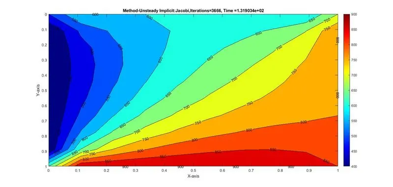
Number of iterations in unsteady methods are way too high compared to steady methods. Here in Jacobi it has taken 3666 iterations to get to stable solution.
Gauss Siedal Method:
Here in the convergence loop iterations are updated in same iterations, that is temperature values of previous points of the same iterations are used to calculate the temperature of the present value of current iteration.
Equation here is
`Tp^(n+1) = (1/(1+2k1 +2k2)) **[(T^(n)p(prev)+k1**(Tl + Tr)^(n+1)+k2** (Tt+ Tb)^(n+1)]`
MATLAB Code for Gauss-Siedal
clear all
close all
clc

%Unsteady State 2D Heat Conduction using Iterative Techniques

%Gauss-Siedal Iterative method

%Inputs
%Dimension of Square Domain
L =1 ;

%No of node points along x-axis
nx = 10;

%No of node points along y-axis
ny = nx;

%discretising
x = linspace(0,L,nx);
y = linspace(0,L,ny);

%Calculating step size dx and dy
dx = x(2)-x(1);
dy = y(2)-y(1);

%Time values
dt = 1e-3;  %Time step
nt = 1400;  %number of time step

%Initialsing error and defining tolerance
error = 9e9;
tol = 1e-4;  % Tolerance value

%Defining Boundary Conditions
%Value of Temperature at Boundaries in K
T_left = 400;
T_right = 800;
T_top = 600;
T_bottom = 900;

%Initialising Temperature at all nodes inside domain
%Initial Condition - Temperature at all nodes is taken 300K
T = 300*ones(nx,ny);

%providing boundary conditions
T( 1:ny, 1) = T_left;
T( 1:ny, nx) = T_right;
T( 1, 1:nx) = T_top;
T( ny, 1:nx) = T_bottom;

%At corners average temperature value is taken
T(1,1) = (T_left + T_top)/2;
T(1,ny) = (T_right + T_top)/2;
T(nx,1) = (T_bottom+T_left)/2;
T(nx,ny) = (T_bottom + T_right)/2;

%Taking Initial T value to a another Array
T_prev = T;
Told = T;

%Defining Thermal Diffusivity Value(alpha) a
a = 1.4;


%Solving Unsteady State equation
%CFL numbers
k1 = a * (dt/dx^2);
k2 = a * (dt/dy^2);

%convergence loop  %Gauss-Siedal Method
gs_iter = 1;

for k = 1:nt      %time loop
    error = 9e9;
    tol = 1e-4;
    while (error > tol)        %Convergence loop

        for i = 2:nx-1          %Spacial loop
            for j= 2:ny-1
                term1 = 1/(1 + (2 * k1) + (2 * k2));
                term2 = k1 * term1;
                term3 = k2 * term1;
                H = T(i-1,j)+ Told(i+1,j);  %left and Right points at older time step
                V = T(i,j-1)+ Told(i,j+1);  %top and bottom points at older time step
                T(i,j) = ( term1 * T_prev(i,j) ) + ( term2 * H ) + ( term3 * V);
            end
        end
        %Inner term max(abs(T-Told)) is an array and maximum value of that array needs to be taken
        error = max(max(abs(T-Told)));
        Told = T;
        gs_iter = gs_iter+1;

    end
    T_prev = T;

end
gs_unsteady_time = toc


figure(1)
%Plotting contour of Temperature

contourf(x,y,T,'showtext','on')  %f is used to get filled contour
%Labelling the lines
% clabel(contourf(x,y,T))
colormap(jet)
colorbar
%Reversing the direction of y-axis
set(gca,'ydir','reverse')
xlabel('X-axis')
ylabel('Y-axis')
title_text = sprintf('Method-Unsteady Implicit:G-S,Iterations = %d, Time =%d',gs_iter,gs_unsteady_time);
title(title_text);
pause(0.03)
Result:
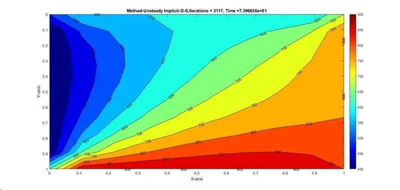
There is a reduction in number of iterations compared to Jacobi but the iterations are too high here also copmpared to steady state method.
SOR Method:
Here the relaxation factor w = 1.2 is used along with Gauss Siedal method as the updated values are used here.
Equation is
`Tp^(n+1) =(1-w)**(T^(n)p) + (w ** (1/(1+2k1 +2k2)) **[(T^(n)p(prev)+k1**(Tl + Tr)^(n+1)+k2** (Tt+ Tb)^(n+1)])`
MATLAB Code for SOR
clear all
close all
clc

%Unsteady State 2D Heat Conduction using Iterative Techniques

%Succesive Over Relaxation(SOR) Iterative method

%Inputs
%Dimension of Square Domain
L =1 ;

%No of node points along x-axis
nx = 10;

%No of node points along y-axis
ny = nx;

%discretising
x = linspace(0,L,nx);
y = linspace(0,L,ny);

%Calculating step size dx and dy
dx = x(2)-x(1);
dy = y(2)-y(1);

%Time values
dt = 1e-3;  %Time step
nt = 1400;  %number of time step

%Initialsing error and defining tolerance
error = 9e9;
tol = 1e-4;  % Tolerance value

%Defining Boundary Conditions
%Value of Temperature at Boundaries in K
T_left = 400;
T_right = 800;
T_top = 600;
T_bottom = 900;

%Initialising Temperature at all nodes inside domain
%Initial Condition - Temperature at all nodes is taken 300K
T = 300*ones(nx,ny);

%providing boundary conditions
T( 1:ny, 1) = T_left;
T( 1:ny, nx) = T_right;
T( 1, 1:nx) = T_top;
T( ny, 1:nx) = T_bottom;

%At corners average temperature value is taken
T(1,1) = (T_left + T_top)/2;
T(1,ny) = (T_right + T_top)/2;
T(nx,1) = (T_bottom+T_left)/2;
T(nx,ny) = (T_bottom + T_right)/2;

%Taking Initial T value to a another Array
T_prev = T;
Told = T;

%Defining Thermal Diffusivity Value(alpha) a
a = 1.4;


%Solving Unseady State equation
%CFL numbers
k1 = a * (dt/dx^2);
k2 = a * (dt/dy^2);

%convergence loop  %SOR Method
%Defining Relaxation Factor omega w
w = 1.2;
sor_iter = 1;

tic
for k = 1:nt      %time loop
    error = 9e9;
    tol = 1e-4;
    while (error > tol)        %Convergence loop

        for i = 2:nx-1          %Spacial loop
            for j= 2:ny-1
                term1 = 1/(1 + (2 * k1) + (2 * k2));
                term2 = k1 * term1;
                term3 = k2 * term1;
                H = T(i-1,j)+ Told(i+1,j);  %left and Right points at older time step
                V = T(i,j-1)+ Told(i,j+1);  %top and bottom points at older time step
                T(i,j) = (1-w) * Told(i,j) + w *(( term1 * T_prev(i,j) ) + ( term2 * H ) + ( term3 * V));
            end
        end
        %Inner term max(abs(T-Told)) is an array and maximum value of that array needs to be taken
        error = max(max(abs(T-Told)));
        Told = T;
        sor_iter = sor_iter+1;

    end
    T_prev = T;

end
sor_unsteady_time = toc

figure(1)
%Plotting contour of Temperature

contourf(x,y,T,'showtext','on')  %f is used to get filled contour
%Labelling the lines
% clabel(contourf(x,y,T))
colormap(jet)
colorbar
%Reversing the direction of y-axis
set(gca,'ydir','reverse')
xlabel('X-axis')
ylabel('Y-axis')
title_text = sprintf('Method-Unsteady Implicit:SOR, Iterations =%d, Time =%d',sor_iter,sor_unsteady_time);
title(title_text);
pause(0.03)
Result:
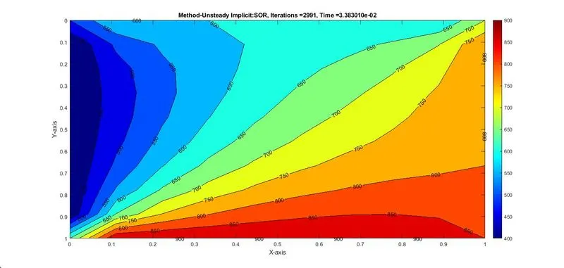
Number of iterations in SOR is 2991 which is less than both jacobi and GS. So it is the enhanced method. Number of iterations may vary according to the relaxation factor provided.
Unsteady – Explicit Method:
In explicit method, the temperature values of previous iterations are used. So all the values are known here to calculate the Temperature value at current time step.
1400 time steps are used and convergence loop is used inside this time loop. Thermal diffusivity term alpha is taken as 1.4.
Equation here is
`Tp^(n+1) =(T^(n)p) + (k1**(Tl -(2**Tp)+Tr)^(n))+(k2** (Tt-(2**Tp)+Tb)^(n))`
k1 and k2 are the CFL values aling x and y axis
`k1= alpha **((Deltat)/(Deltax^2))`
`k2= alpha **((Deltat)/(Deltay^2))`
and summation of this needs to be less than 0.5 for stable solution.
MATLAB Code for Unsteady-Explicit Method:
clear all
close all
clc

%Unsteady State 2D Heat Conduction using Explicit Method

%Explicit method

%Inputs
%Dimension of Square Domain
L =1 ;

%No of node points along x-axis
nx = 10;

%No of node points along y-axis
ny = nx;

%discretising
x = linspace(0,L,nx);
y = linspace(0,L,ny);

%Calculating step size dx and dy
dx = x(2)-x(1);
dy = y(2)-y(1);

%Time values
dt = 1e-3;  %Time step
nt = 1400;  %number of time step

%Initialsing error and defining tolerance
error = 9e9;
tol = 1e-4;  % Tolerance value

%Defining Boundary Conditions
%Value of Temperature at Boundaries in K
T_left = 400;
T_right = 800;
T_top = 600;
T_bottom = 900;

%Initialising Temperature at all nodes inside domain
%Initial Condition - Temperature at all nodes is taken 300K
T = 300*ones(nx,ny);

%providing boundary conditions
T( 1:ny, 1) = T_left;
T( 1:ny, nx) = T_right;
T( 1, 1:nx) = T_top;
T( ny, 1:nx) = T_bottom;

%At corners average temperature value is taken
T(1,1) = (T_left + T_top)/2;
T(1,ny) = (T_right + T_top)/2;
T(nx,1) = (T_bottom+T_left)/2;
T(nx,ny) = (T_bottom + T_right)/2;

%Taking Initial T value to a another Array
T_prev = T;
Told = T;

%Defining Thermal Diffusivity Value(alpha) a
a = 1.4;


%Solving Unsteady State equation
%CFL numbers
k1 = a * (dt/dx^2);
k2 = a * (dt/dy^2);

%convergence loop  %Explicit Method for Unsteady
explicit_iter = 1;

tic
for k = 1:nt      %time loop
    error = 9e9;
    tol = 1e-4;
    while (error > tol)        %Convergence loop

        for i = 2:nx-1            %Spacial loop
            for j= 2:ny-1
                H = Told(i-1,j)-(2 * Told(i,j))+ Told(i+1,j);  %left and Right points at older time step
                V = Told(i,j-1)-(2 * Told(i,j)) + Told(i,j+1); %top and bottom points at older time step
                T(i,j) = ( Told(i,j) ) + ( k1 * H ) + ( k2 * V);
            end
        end
        %Inner term max(abs(T-Told)) is an array and maximum value of that array needs to be taken
        error = max(max(abs(T-Told)));
        Told = T;
        explicit_iter = explicit_iter+1;

    end
                          %No need of updating T_prev
end
explicit_unsteady_time = toc


figure(1)
%Plotting contour of Temperature

contourf(x,y,T,'showtext','on')  %f is used to get filled contour
%Labelling the lines
% clabel(contourf(x,y,T))
colormap(jet)
colorbar
%Reversing the direction of y-axis
set(gca,'ydir','reverse')
xlabel('X-axis')
ylabel('Y-axis')
title_text = sprintf('Method-Unsteady Explicit, Iterations =%d, Time =%d',explicit_iter,explicit_unsteady_time);
title(title_text);
pause(0.03)
Result:
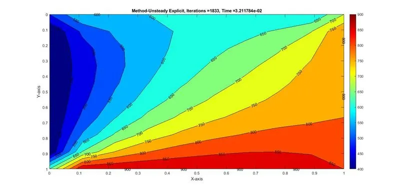
Number of iterations here is 1883 and is lesser than the iterative methods.
Conclusion:
1. Order of number of Iterations in Steady State Heat Conduction is as follows.
Number of iterations in of (Jacobi > Gauss Siedal > SOR) method and it tells us that SOR is better one.
2. The number of iterations in Unsteady Explicit method are lesser than Implicit Iterartive Methods.
3. in Unsteady/Transient State heat conduction method, number of iterations in all iterative methods are larger than Steady State heat conduction and order of number of iterations is as follows.
Number of iterations of (Jacobi > Gauss Siedal > SOR ) and also here SOR is enhanced solver.
4. Temperature contour is plotted for all different states and methods. The process of heat conduction through body of 1 * 1 dimensions with prescribed boundary and initial conditions is studied. Temperature variation within domain and values after attaining stable solution are analysed.