Week 5: Prandtl Meyer Shock problem
Aim:
To simulate the Prandtl - Meyer shock flow problem using Converge
To setup the problem for supersonic and subsonic flows near the convex corner or sharp corner and study the change in flow variables
To study the effect of SGS tempertaure value on cell count, shock location and production of Mesh.
To understand different types of Boundary conditions used in CFD and shock flow problems.
Boundary Conditions:
Boundary conditions are the constraints necessary for the solution of a boundary value problem. Both ordinary and partial differential equations need boundary conditions to be solved. Different type of boundary conditions can be imposed on the boundary of the Domain. The choice of the boundary condition is fundamental for the resolution of the computational problem. A bad imposition of the boundary condition may lead to the divergence of the solution or convergence to the bad solution.
There are 5 types of Boundary Conditions:
Dirichlet BC: This condition specifies the value of the variable at a boundary. It is also called a fixed function. So it is used when a value needs to be imposed along the boundary of the domain.
Neumann BC: This condition specifies the values that the derivative of a solution is going to take on the boundary of the domain.
`(du)/(dx) = f(x)`
Robin’s BC: It consists of a linear combination of the values of the field and its derivatives on the boundary. So it is a linear combination of Dirichlet and Neumann boundary condition applied to an entire boundary.
`aφ(x)+b(∂φ)/(∂x)=f(x)` where a and b are real parameters. This condition is also called impedance conditio.
Mixed BC: It consists of applying different types of boundary conditions in different parts of the domain. The mixed boundary condition differs from the Robin condition because the latter consists of different types of boundary conditions applied to the same region of the boundary, while the mixed condition implies different types of bondary condition applied to different parts of the boundary.
Cauchy BC: The Cauchy boundary condition is a condition applied on both the unknown variable and its derivatives. It differs from the Robin condition because the Cauchy condition implies the imposition of two constraints (1 Dirichlet boundary condition and 1 Neumann boundary condition), while the Robin condition implies only one constraint on the linear combination of the unknown function and its derivatives.
Shock Wave
Shock wave or shock, is a type of propagating disturbance that moves faster than the local speed of sound in the medium. Like an ordinary wave, a shock wave carries energy and can propagate through a medium but is characterized by an abrupt, nearly discontinuous, change in pressure, temperature, and density of the medium.
When the speed of the moving object exceeds the speed of the sound in a medium, then wavefront lag behind the object forming a cone shaped region with the source behind the object. The edge of the cone forms supersonic wavefront with a large amplitude which is called as shock wave.
Shock wave, strong pressure wave in any elastic medium such as air, water, or a solid substance, produced by supersonic aircraft, explosions, lightning, or other phenomena that create violent changes in pressure. Shock waves differ from sound waves in that the wave front, in which compression takes place, is a region of sudden and violent change in stress, density, and temperature. Because of this, shock waves propagate in a manner different from that of ordinary acoustic waves.
Shock waves can be:
Normal
At 90° (perpendicular) to the shock medium's flow direction.
Oblique
At an angle to the direction of flow.
Bow
Occurs upstream of the front of a blunt object when the upstream flow velocity exceeds Mach 1.
Mach Number:
Mach number is the ratio of the speed of a moving object to the local speed of sound. It is a dimensionless number. Speeds less than the speed of sound have a Mach number between zero and one and are described as subsonic. Those greater than the speed of sound have Mach numbers greater than one are a described as supersonic. Speeds approximately equal to the speed of sound have Mach numbers approximately equal to one and are described as transonic. In the current problem velocity of 680 m/s at 286.1 K is used which is around 2 Mach and supersonic.
Prandtl–Meyer Expansion fan
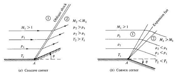
A supersonic expansion fan, technically known as Prandtl–Meyer expansion fan, a two-dimensional simple wave, is a centered expansion process that occurs when a supersonic flow turns around a convex corner. The fan consists of an infinite number of Mach waves, diverging from a sharp corner. Each wave in the expansion fan turns the flow gradually (in small step). The expansion fan consists of an infinite number of expansion waves or Mach lines
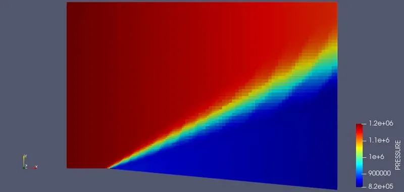
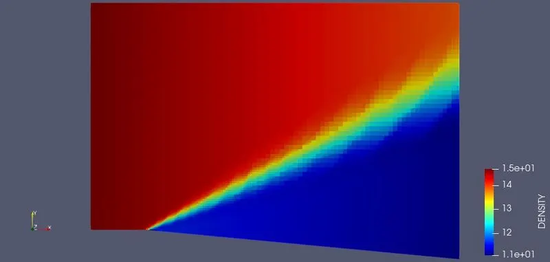
Across the expansion fan, the flow accelerates (velocity increases) and the Mach number increases, while the static pressure, temperature and density decrease. Since the process is isentropic, the stagnation properties (e.g. the total pressure and total temperature) remain constant across the fan.
Zero Gradient:
zeroGradient boundary condition extrapolates the quantity to the boundary from the nearest cell value. Zero normal gradient means the quantity is developed in space and its gradient is equal to zero in direction perpendicular to the boundary.
zero gradient value boundary conditions are Neumann boundary conditions.
slip boundary condition: The velocity normal to the boundary is set to zero, while the velocity parallel to the boundary is let free.
Why Neumann BC are used in this problem (Supersonic/ Shock flows)
Since values of the variables (Pressure, velocity, Temperature etc) are not available before solving this supersonic flow problem, nothing is specified at supersonic outlet and all these variables are extrapolated from the interior domain or nearest cells to the boundary. Only the normal derivative of variables ( normal wrt outlet boundary) are specied as 0 (Zero normal Gradient).
Setting up Simulation:
Initially the STL file of the geometry is imported and scaled down to 0.001. Then the normal of the triangles are turned on. If they are poiniting outwards, go to Tansform > Normal > select any triangle and hit apply as they should be pointing inwards for this simulation.
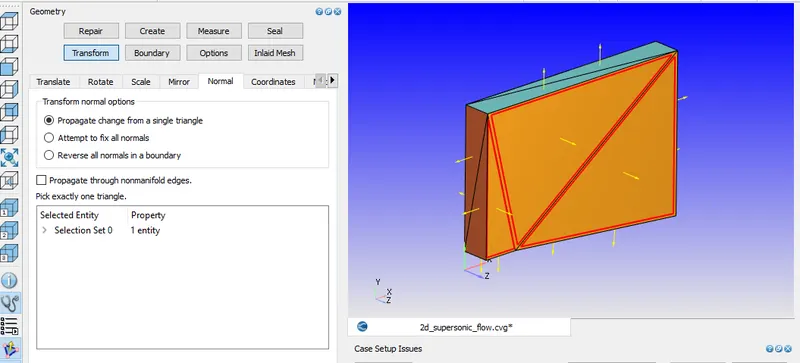
Run diagnosis, if there are no errors then go to Boundary > Flag > Create multiple Boundaries to flag the different boundaries to the geometry.
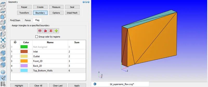
The geometry looks like above after creating Inlet, Outlet ,Top-Bottom_Walls, Front and Bacl Boundaries.
Lx = 65 m
Ly = 45.15 m
Lz = 8.15 m
Case Setup:
1. Applications type: Time - Based
2. Materials:
Select default values for Gas Simulation and Global Transport Properties.
Species : Add N2 and O2 in Gas
3.Initial Condition and Events:
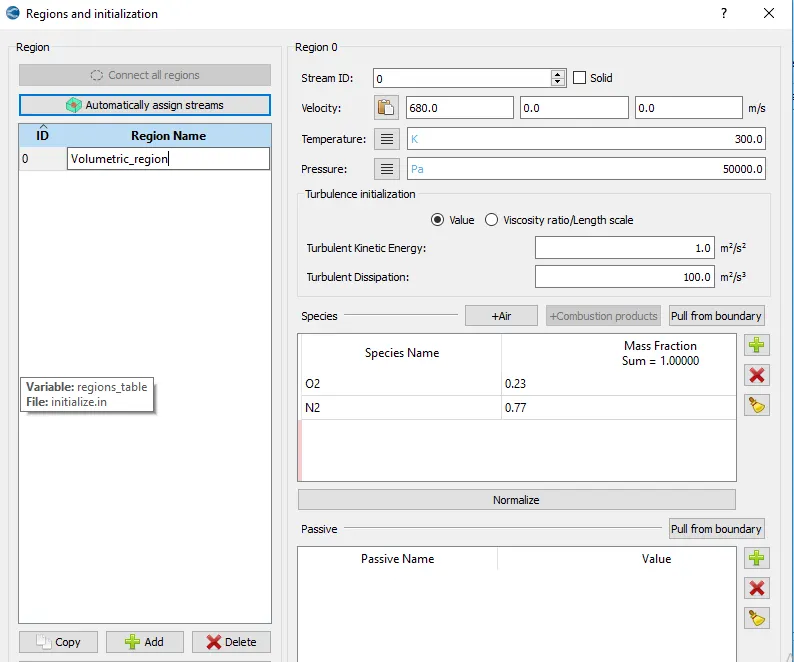
Add a region as Volumetric_Region in regions and Initialisation and intialise species value with below mass fraction
O2 - 0.23
N2 - 0.77 whose combination makes the Air as the working fluid for simulation.
Velocity is set to 680m/s along x-axis and below mentioned values are applied to temperature and pressure.
4. Boundary Conditions:
Inlet
Boundary type - INFLOW.
Velocity - 680 m/s along X-axis so the problem includes supersonic Inlet
Temperature - 286.1 K . This temperature makes the velocity of 680 m/s to mach number of 2 making the flow supersonic
Species - N2 = 0.77 and O2 = 0.23
select Volumetric_region as region for all boundaries.
Pressure BC is Zero normal gradient which is Neumann Boundary condition.
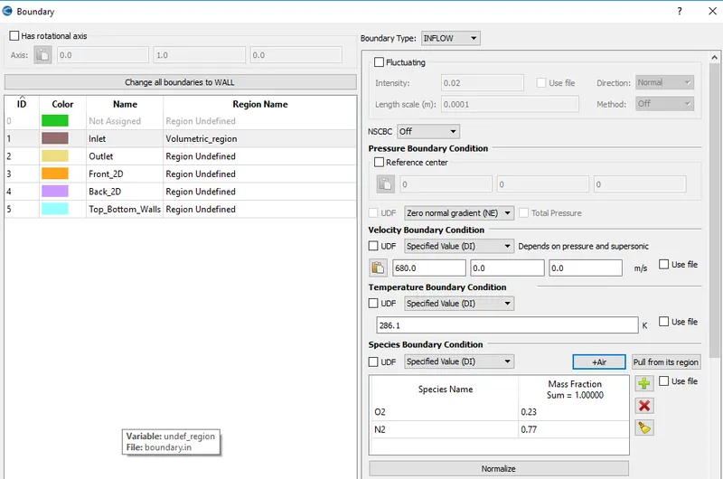
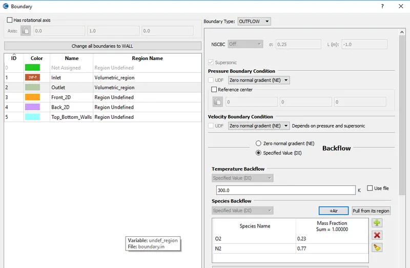
Outlet
Boundary type - OUTFLOW.
Temperature - 300 K
Species - N2 = 0.77 and O2 = 0.23
.Also mention O2 and N2 species dor Backflow ( if it occurs due to adverse pressure)
Pressure and Velocity BC is Zero normal gradient which is Neumann Boundary condition.
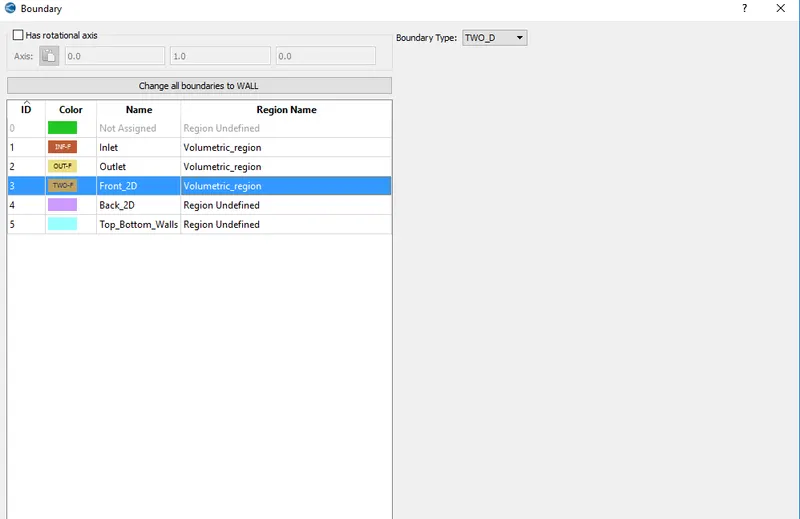
Front_2D:
Boundary type is TWO_D
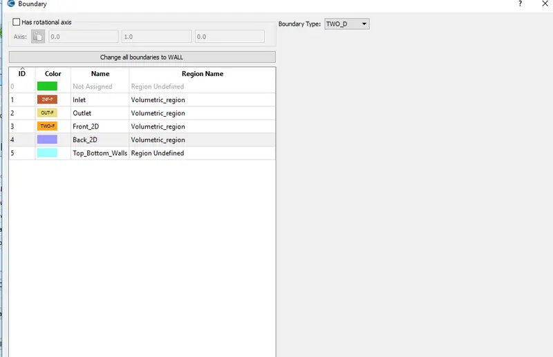
Back_2D:
Boundary type is TWO_D
Top_Bottom_Walls:
Boundary type is wall. Slip condition is applied so that variable values in the cells near walls will not be same as walls.
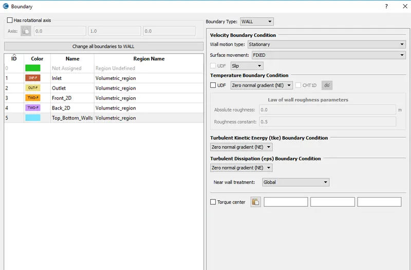
Zero normal gradient (Neumann BC) is applied for all the boundary conditions at Outlet and Wall in the problem since the flow is supersonic and it is hard to calculate the values before hand. So the values at these boundaries are calculated from the cells near them when zero normal gradient condition is applied.
5. Simulation Parameters:
Run parameters:
Solver : Steady- State solver
Simulation mode: Full hydrodynamic
Turn off use shared memory and turn on steady state monitor Misc tab.
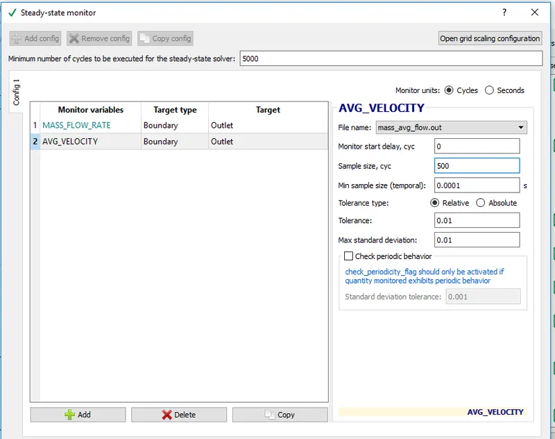
Steady State Monitor:
Add required parametres that need to be monitored so that if they converge within the given tolerance value the simulation would stop before reaching the given number of cycles to complete(End time)
Simulation Time Parameters:
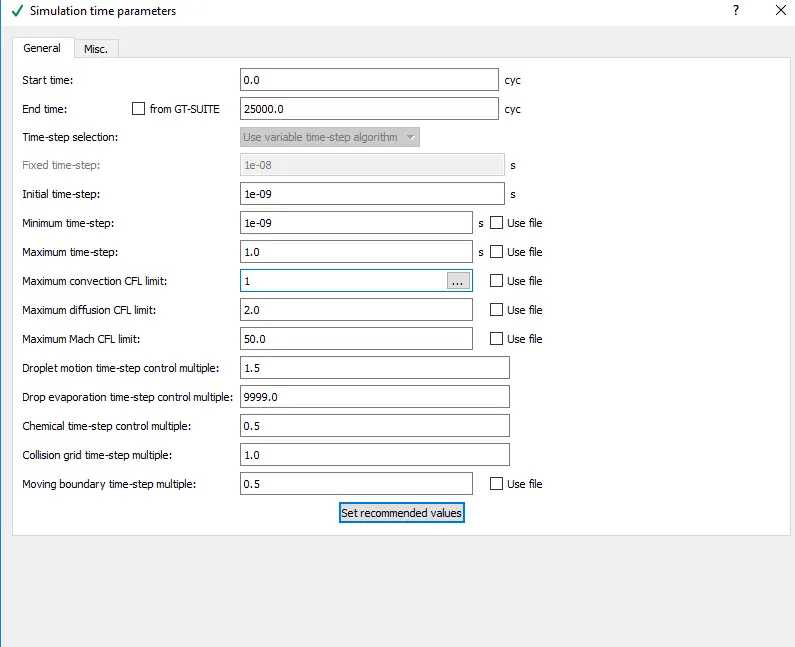
Start time - 0
End time - 25000 cycles
Intial time step : 1e-9 s
Minimum time step:1e-9 s
Maximum Time step: 1 s
Maximum convection CFL limit: 1
Leave the rest as Default values.
Solver Parameters:
NS solver Scheme - PISO
NS Solver Type - Density Based Steady as Density of fluid will be changing inside the geomtery
Set the pre conditioner to none in Pressure in the Equation tab.
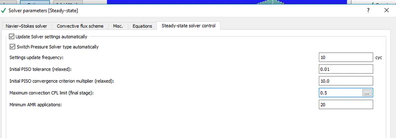
Set the maximum convection CFL limit to 0.5 in Steady state Solver Control tab and rest are left Default.
6. Physical Models:
Turbulence model : RNG k -`epsilon` in RANS
7. Grid Control :
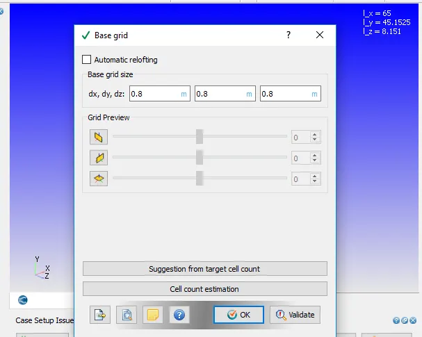
Base grid : dx=dy=dx = 0.8 m
Add Adaptive Mesh Refinement in Grid control
Adaptive Mesh Refinement:
We need finer mesh to capture the accurate values of the varibales. I this current proble, the values will vary a lot after flow passes through the sharp corner in the geometry. So in order to capture the accurate results there we need smaller and finer mesh in that region. Making the mesh size smaller in the whole geometry will lead to large number of cells and it is unnecesary. So we will make use of a technique called Adaptive Mesh Refinement. The technique makes the geomtery finer only in certain region where the given conditions satisfies capturing the accurate results with lesser number of cells. In this problem we make use temperature varibale which refines the mesh based on the variation of temperature between the cells. Sub-Grid Scale criterion is used for Embed type with embedding level of 2. The given value of sub-grid criterion is 0.05 K. So if `(del^2T)/(dx)^2` > 0.05 K, between any cells, the mesh will be refined in that region. the refined mesh size will be
`REFINED Mesh Size = (Base Mesh)/ (2^(EMBEDD LEVEL))`
which reduces the mesh size 0.2m(as base mesh is 0.8m) in the region where `(del^2T)/(dx)^2` > 0.05, (in two levels, 0.4 m in ouer layer and 0,2 m in inner layer) thereby refining the mesh and keeping base mesh at remaining regions
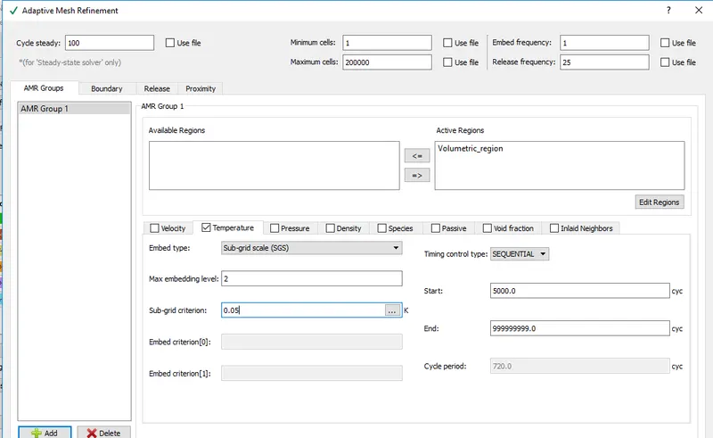
Three simulations are ran with doifferent values of SGS(Sub-Grid Scale) to study its effect on the number of cells and the accuracy of the solution.
SGS value of 0.08, 0.05 and 0.01K are used for simulations and those regions which have values below than these values will be refined.
8. Output/Post-processing
In post variable selection, under SPecies tab, add N2 and O2 in mass fraction box.
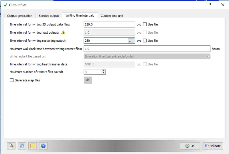
In output files, under Writing time intervals tab, specify 250 cycles as time interval for writing 3D output data files and restarting files yo get 100 files for post processing.
Export All these input files to a directory. Open CYGWIN, navigate to the directory where all these folders are saved and run the following command ;
mpiexec.exe -n 4 converge.exe restricted logfile_006 &
which runs the simulation with 4 processors using converge executable and outputs are dumped into a file called logfile_006 with job being ran in backend.
Outputs/Post -Processing:
Post processing is performed in the paraview software using the group files with ..vtm extension created in the post processor of Converge
Case -1 : Base Mesh - 0.8m SGS(Sub-Grid Scale) - 0.08 K Inlet Velocity - 680m/s
Mesh:
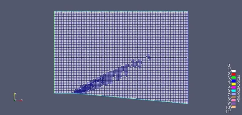
Refinenment of mesh for some extent at sharp corner can be seen. Since the value of SGS is quite high, refinement region is not much. For values of `(del^2T)/(dx)^2` > 0.08, mesh will be refined
Temperature Contour:
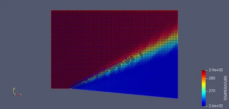
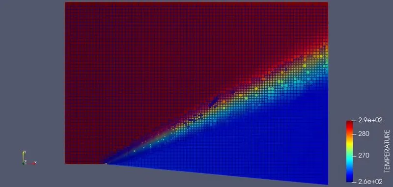
Temperature reduces past the corner till outlet. There is large variation of temperature after the corner. Its around 261 K at outlet.
Pressure Contour:
Density Contour:
Velocity Contour:
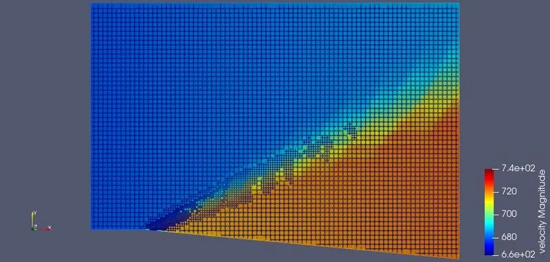
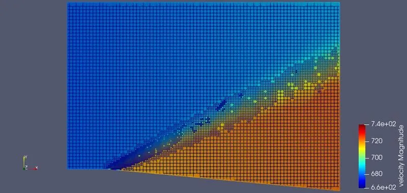
Velocity increases past the sharp corner at some angle to the horizontal there by increasing the mach number at the outlet. This process is called expansion and all other variables pressure, density and temperature can be seen reducing in the regions where there is increase in the velocity.
Mach Number:
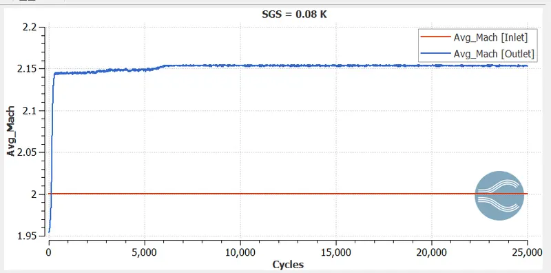
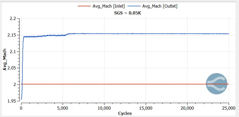
For the supersonic inlet velocity, after the expansion process at sharp corner, velocity increases and Mach number can be seen rasied by value of 0.15 at Outlet than inlet.
Total Number of Cells:
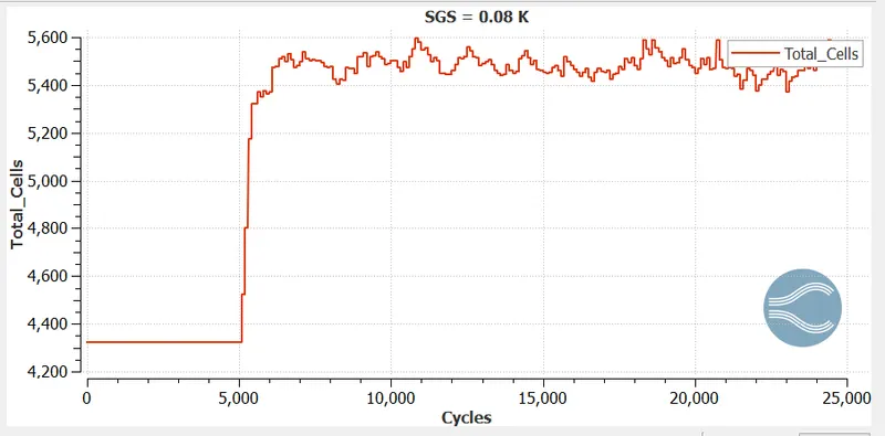
After 5000 cycles, when adaptive mesh refinement starts, we can see the sudden increase in the cell numbers since the mesh is getting refined due to tempertaure difference between two cells is less than the prescribed value in some regions. Total number of cells fluctuates between 5400 to 5600.
Case -2 : Base Mesh - 0.8m SGS(Sub-Grid Scale) - 0.05 K Inlet Velocity - 680m/s
Mesh:
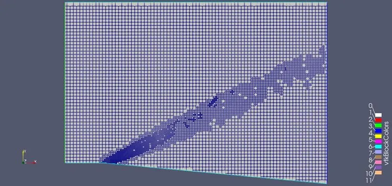
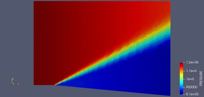
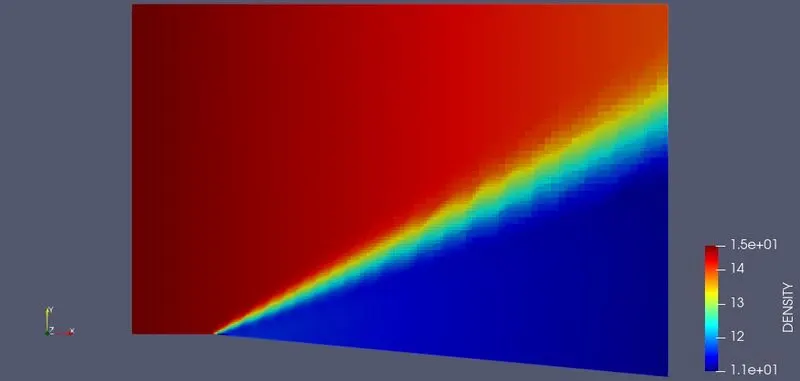
When there is reduction in the SGS value for 0.05, we can see the mesh getting refined for higher region than the previous case. For all the values where the `(del^2T)/(dx)^2` > 0.05, the mesh gets refined. the refinement region is after the sharp corner where there is major change in the flow variables.
Temperature Contour:
Pressure Contour:
Density Contour:
Velocity Contour:
Mach Number:
Total number of Cells:
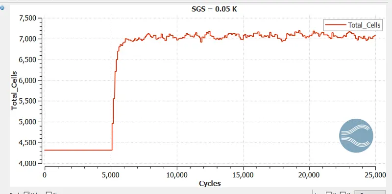
we can see there is increase in the number of cells in this case than the previous one. Since SGS parameter is reduced, any value above it will lead to refinement in mesh thereby increasing the mesh size. The number of cells is around 7000 to 7100.
Case -3 : Base Mesh - 0.8m SGS(Sub-Grid Scale) - 0.05 K Inlet Velocity - 100m/s
Subsonic Inlet:
Mesh:
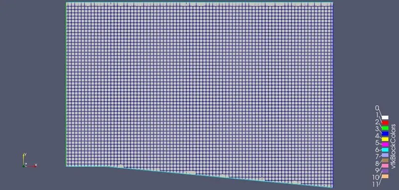
We can see that for subsonic inlet, there is not change in the flow variables at cell level compared to supersonic inlet. So the adavptive mesh refinement will not take place even thougfh the SGS parameter is 0.05. We can see the temperature variation after flow passes through sharp corner is not at cell level and it decreases by 2K.
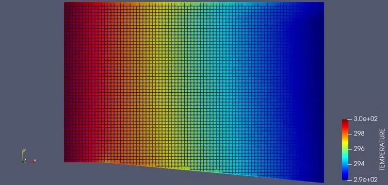
Temperature variation is not at cell level as in case of supersonic inlet. So we can say that expanison process takes place for supersonic inlet. Temperature decreases from inlet to outlet and the difference is around 8K.
Pressure Contour:
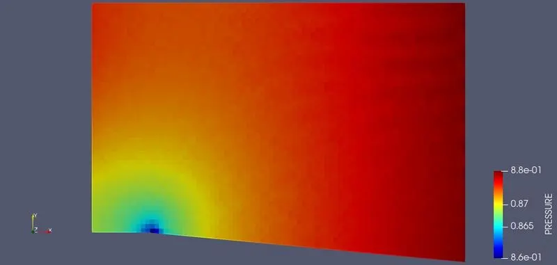
There is small variation of pressure at the corner and pressure is lower at the corner. Since there is decrease in the velocity of the fluid past the corner, to compensate drop in the velocoity, pressure can be seen rising at the outlet.
Density contour:
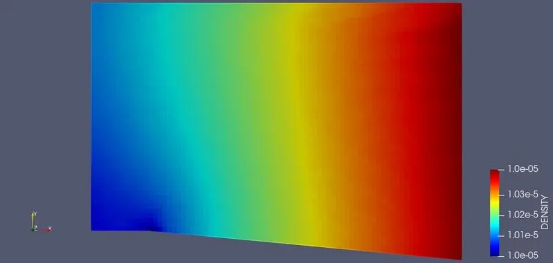
Density also increases past the corner and the behaviour oif variation of density in this case is opposite to that of supersonic inlet.
Velocity Contour:
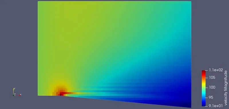
Velocity is quite high at the corner and reduces past the corner and the behaviour is opposite to the supersonic inlet. The velocity at the outlet is less than the inlet and we can say expansion process doesnt takes place in this case. This drop of velocity leads to rise in the static pressure there by maintaining the equal total pressure at inlet and outlet.
Mach Number:
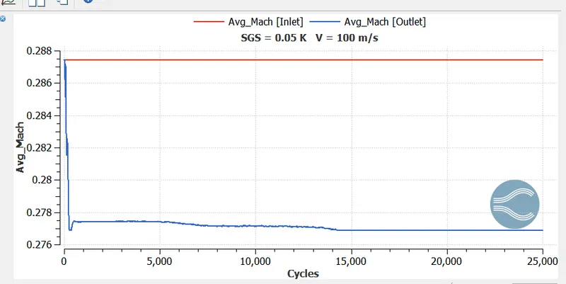
We can see there is reduction in the mach number at the outlet. As opposed to the supersonic inlet, the flow velocity reduces after the sharp corner in the geometry in the subsonic case.
Total Number of Cells:
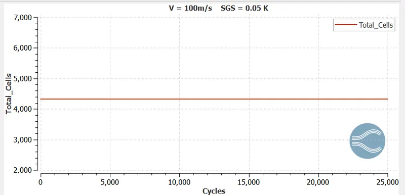
Since there is no mesh refinement as the Temperature variation is not in the cell level, the mesh remains uniform throughtout the geometry, mesh size is constant making the cell number equal throughout the simulation and it is around 4400.
Case -4 : Base Mesh - 0.8m SGS(Sub-Grid Scale) - 0.01 K Inlet Velocity - 680m/s
In this case the Inlet is again made supersonic and the SGS value is further reduced to 0.01K to obtain the improved mesh and results.
Mesh:
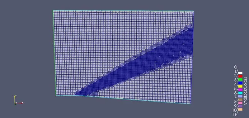
Mesh refinement is high good quality and mesh is refined in larger area for decreases SGS value. So we can say lower the SGS, higher the cell size and fner the mesh.
Temperature Contour:
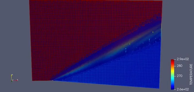
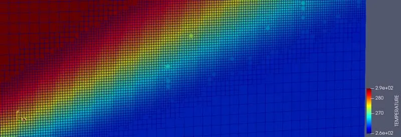
Variation of the temperature can be seen in layers at some angles to horizontl. So the shock waves are produced due to the corner and are inclined at some angles to horizontal. The contour can be seen clearly below
Pressure Contour:
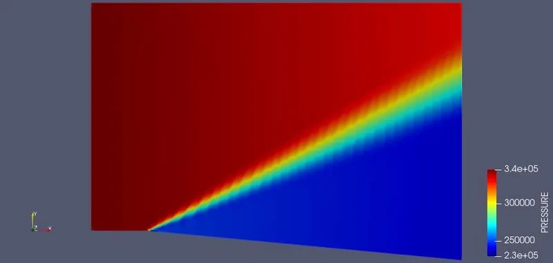
Denisty Contour:
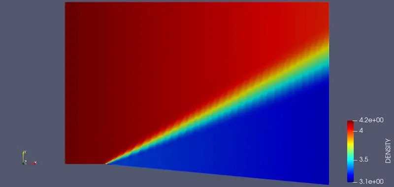
Pressure and density reduces past the corner and in thiose regions where the velocity is increased.
Velocity Contour:
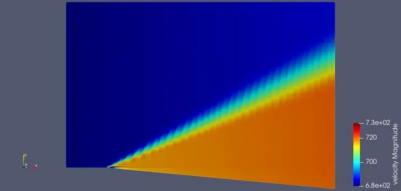
The inlet velocity is 680m/s and the outlet velocity is around 730 m/s and we can say the expansion of the flow has taken place past the corner where all other properties except velocity decreases. Shock waves are produced at some angles to the horizontal across which the fluid properties varies. Increase in the velocity increases the outlet mach number and can be seen below.
Mach number:
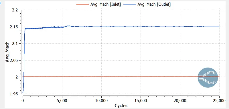
Mach number increases at the outlet and is equal to 2.15.
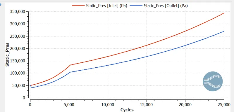
Static Pressure:
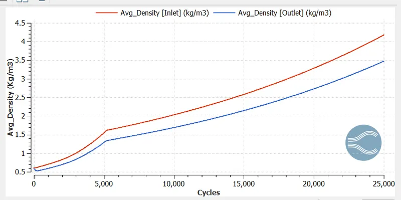
Average Density:
Temperature:
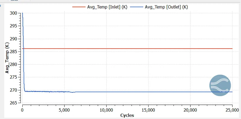
We can see the reduction in the static pressure, temperature and density at the outlet. Since the flow expands past the corner, the number of particles in a volume reduces thereby decreasing the density and making the flow compressible one. Due to incrase in the velocity, static pressure drops past the corner till outlet.
Total Pressure:
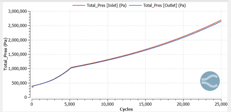
Though there are large variation in the fluid properties past teh corner for supersonic inlet, the total pressure remains almost constant in the system and is nearly equal at inlet and outlet. The static pressure drops past corner, but since there is increase in the velocity and it leads to increase in dynamic pressure which compensates for drop in static pressure makin the toatl pressure constant.
Total number of Cells:
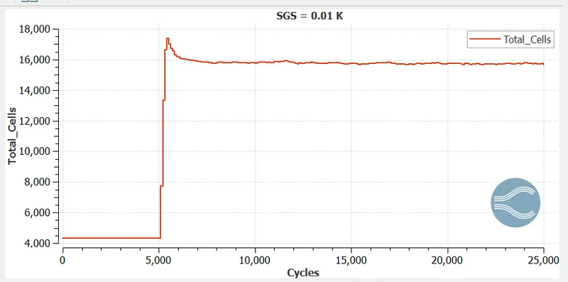
The mesh is much finer than all the cases. So the number of cells is higher than remaining cases and is around 16000 after 5000 cycles when adaptive mesh refinement based on temperature starts.
Animations:
1. SGS - 0.08 K Inlet Velocity - 680m/s
Animation of Temperature Contour:
2. SGS - 0.05 K Inlet Velocity - 680m/s
Animation of Temperature Contour:
3. SGS - 0.05 K Inlet Velocity - 100m/s
Animation of Temperature Contour:
4. SGS - 0.01 K Inlet Velocity - 680m/s
Animation of Mesh production and Adaptive Mesh Refinement:
Animation of Temperature Contour:
Animation depicts the Prandtl - Meyer shock analysis problem. The inlet velocity is 680 m/s which is 2 Mach at 286.1 K and is supersonic. When this flow is made to pass through the convex or sharp corner in the geometry, flow expansion take place leading to production of shock waves which is inclined at some angles to horizontal across which the fluid properties varies. Velocity and mach number increases and there is decrease in pressure, temperature and density. Accurate results are captured with finer mesh in this region using the Adaptive Mesh refinement technique in Converge. When the temperature difference between two cells is higher than the prescribed SGS ( here 0.01 K), mesh refinement takes place and reduced by 4 times than the base mesh size increasing total number of cells. Animations are saved in Paraview. Zoomed animation at the shock region and variation of temperature there can be seen below.
Conclusion:
Studied the behaviour of flow variables (velocity, Temperature, Pressure, denisty and Mach number) when the fluid flow past the sharp corner in the geometry.
For supersonic inlet velocity, the Variables Velocity and Mach number increases past the corner till the outlet and all other variables reduces so there by maintaining the constant total pressure. The behaviour is opposite for the subsonic inlet here velocity reduces and other variables increase past the corner.
For supersonic inlet, we can say the expansion process takes place past the corner producing the shock waves at some angle to the horizontal across which the velocity of the fluid increases increasing the mach number and reducing pressure, density and temperature.Total pressure remains constant in the system. Studied the production of Shock waves for supersonic inlets.
Studied the effect of Temperature SGS criterion on thh refinement of mesh. For a given value of SGS , if the difference between the adjacent cells is higher than give SGS, we can see the mesh refinement in that region. The base mesh size is 0.8 m and refinement takes place at two levels with 0.4m in outside layer and 0.2m mesh size inside.
Lower the value of the Temperature SGS, the higher the cell number, making the mesh finer in large area thereby the capturing the values accurately and increasing the simulation time.