Week 3.5 - Deriving 4th order approximation of a 2nd order derivative using Taylor Table method
Aim:
Derive the 4th order approximations of the second-order derivative with
- Central difference
- Skewed right-sided difference
- Skewed left-sided difference
Using Taylor table method and to compare the errors involved in the schemes using MATLAB
Theory:
Second order derivative of analytical function can be determined by the numerical methods of second or fourth orders. Here fourth order approximation is used to determine the second derivative of the function and the difference between the solutions is calculated as error and the accuracy of the method is evaluated using that error. The approximations are fourth order because the truncation error involved in the schemes is of fourth order.
Given
The order of accuracy P= Number of nodes in the stencil N - order of derivative Q + 1 for symmetric/central schemes
From this we can derive
Number of nodes in the stencil N = P+Q-1
Here, P =4
Q =2
Hence number of nodes for symmetric/central schemes = (4+2-1) = 5
These nodes can be represented as
x-2dx, x-dx, x, x+dx, x+2dx when the central node is x and the remaining are neighbour nodes.
- ii) The order of accuracy P= Number of nodes in the stencil N- order of derivative Q for one-sided/skewed schemes
Number of nodes in the stencil N = P+Q
Here, P =4
Q =2
Hence number of nodes for skewed schemes = (4+2) = 6
These 6 nodes can be represented in skewed right scheme as
x, x+dx, x+2dx, x+3dx, x+4dx, x+5dx where x is out first node and remaining are nodes right to it.
This is same for skewed left scheme but neighbor nodes are left to it.
Deriving the Schemes:
Central Difference Scheme:
The function at nodes can be written as
f(x-2dx), f(x-dx), f(x), f(x+dx), f(x+2dx)
Second order derivative in central differencing can be written as
`(Deltax)^2(d^2f)/dx^2 = a*f(x-2dx) + b*f(x-dx) +c*f(x) + d*f(x+dx) + e* f(x+2dx)`
| f(x) | `f'(x)*Deltax` | `f''(x)*(Deltax)^2` | `f'''(x)*(Deltax)^3` | `f^(iv)(x)*(Deltax)^4` | `f^v(x)*(Deltax)^5` | `f^(vi)(x)*(Deltax)^6` | |
| a*f(x-2dx) | a | -2a | `4/2a` | `-8/6a` | `16/24a` | `-32/120a` | `64/720a` |
| b*f(x-dx) | b | -b | `b/2` | `-b/6` | `b/24` | `-b/120` | `b/720` |
| c*f(x) | c | 0 | 0 | 0 | 0 | 0 | 0 |
| d*f(x+dx) | d | d | `d/2` | `d/6` | `d/24` | `d/120` | `d/720` |
| e*f(x+2dx) | e | 2e | `4/2e` | `8/6e` | `16/24e` | `32/120e` | `64/720e` |
| `sum` | 0 | 0 | 1 | 0 | 0 | 0 | ? |
From the above table 5 equations can be formed to solve 5 unknowns.
`a+b+c+d+e= 0`
`-2a-b+0+d+2e = 0`
`2a + b/2 + 0 + d/2 + 2e = 1`
`-8/6a-b/6+0+d/6+8/6e = 0`
`16/24a +b/24=0+d/24+16/24e = 0`
Solving these in MATLAB gives the values of unknown as
a= -0.083333
b = 1.3333
c = -2.5
d = 1.3333
e = -0.083333
Along `f^v(x)*(Deltax)^5` the column the positive and negative coefficients cancel each other. So the remaining terms in the equation are
`(Deltax)^2*(d^2f)/dx^2 = [2a +b/2+0+d/2+2e]f''(x)*(Deltax)^2+{64/720a+b/720+0+d/720+64/72-e]f^(vi)(x)*(Deltax)^6`
Dividing both sides by `(Deltax)^2` we get
`(d^2f)/dx^2 = [2a +b/2+0+d/2+2e]f''(x)+{64/720a+b/720+0+d/720+64/72-e]f^(vi)(x)*(Deltax)^4`
So ignoring the last term having `(Deltax)^4`, we het our required equation and since we ignored `(Deltax)^4`, the approximation is called fourth order central differencing approximation.
and substituing the values of a,b,c,d and e we get the approximation for Second order derivative using central differencing as
`(d^2f)/dx^2 = (-0.0833*f(x-2dx) + 1.3333*f(x-dx) -2.5*f(x) + 1.3333*f(x+dx) -0.0833* f(x+2dx))/(Deltax)^2`
Given analytical function is f(x)= exp(x)*cos(x)
Differenciating the function twice with respect to x, we get
f'(x) = exp(x)*(-sin(x)) + exp(x)*cos(x)
f''(x) = exp(x)*(-cos(x)) + exp(x)*(-sin(x)) + (exp(x)*cos(x)) + exp(x)*(-sin(x))
f''(x) = -(2 * exp(x) * sin(x))
Function for Central differencing in MATLAB:
  function error_central = central_diff(analytical_derivative,x,dx);

    %4th order approximation of 2nd order Derivative
    %Central Differenicing Scheme

    %Coefficient Matrix
    A = [1 1 1 1 1; -2 -1 0 1 2; 2 1/2 0 1/2 2; -8/6 -1/6 0 1/6 8/6; 16/24 1/24 0 1/24 16/24;];
    B = [0; 0; 1; 0; 0;];

    %Solution for central differnece
    C = inv(A)* B;

    %d^2f/dx^2 = a*f(x-2dx) + b*(f-dx) + c*f(x) + d*f(x+dx) + e*f(x+2dx)
    %analytical function f(x) = exp(x)*cos(x)
    fourth_central = (C(1)*(exp(x-2*dx)*cos(x-2*dx)) + C(2)*(exp(x-dx)*cos(x-dx)) + C(3)*(exp(x)*cos(x)) + C(4)*(exp(x+dx)*cos(x+dx)) + C(5)*(exp(x+2*dx)*cos(x+2*dx)))/(dx^2);
    error_central = abs(analytical_derivative - fourth_central);

  endfunction
Skewed Right Sided Difference Scheme:
Using the formula for number of nodes, we get 6 nodes in the stencil. These nodes in the function form can be written as
f(x), f(x+dx), f(x+2dx), f(x+3dx), f(x+4dx), f(x+5dx). x is the initial node and remaining are right to it with equally spaced distance dx between them.
Second order derivative in skewed right sided differencing can be written as
`(Deltax)^2(d^2f)/dx^2 = a*f(x) + b*f(x+dx) +c*f(x+2dx) + d*f(x+3dx) + e* f(x+4dx)+g*f(x+5dx)`
Writing these terms in Taylor table after expansion of each term
| f(x) | `f'(x)*Deltax` | `f''(x)*(Deltax)^2` | `f'''(x)*(Deltax)^3` | `f^(iv)(x)*(Deltax)^4` | `f^v(x)*(Deltax)^5` | `f^(vi)(x)*(Deltax)^6` | |
| a*f(x) | a | 0 | 0 | 0 | 0 | 0 | 0 |
| b*f(x+dx) | b | b | `b/2` | `b/6` | `b/24` | `b/120` | `b/720` |
| c*f(x+2dx) | c | 2c | 2c | `8/6c` | `16/24c` | `32/120c` | `64/720c` |
| d*f(x+3dx) | d | 3d | `9/2d` | `9/2d` | `27/8d` | `81/40d` | `243/240d` |
| e*f(x+4dx) | e | 4e | `8e` | `32/3e` | `32/3e` | `128/15e` | `512/90e` |
| g*f(x+5dx) | g | 5g | `25/2g` | `125/6g` | `625/24g` | `3125/120g` | `15625/720g` |
| `sum` | 0 | 0 | 1 | 0 | 0 | 0 | ? |
From the above table 6 equations can be formed to solve 6 unknowns.
`a+b+c+d+e+g= 0`
`0+b+2c+3d+4e+5g = 0`
`0+b/2+2c+9/2d+8e+25/2g = 1`
`0+b/6+8/6c+9/2d+32/3e+125/6g = 0`
`0+b/24+16/24c+27/8d+32/3e+625/24g = 0`
`0+b/120+32/120c+81/40d+128/15e+3125/120g = 0`
So the remaining terms in the equation are
`(Deltax)^2*(d^2f)/dx^2 = [0 +b/2+2c+9/2d+8e+25/2f]f''(x)*(Deltax)^2+[0+b/720+64/720c+243/240d+512/90e+15625/720g]f^(vi)(x)*(Deltax)^6`
Dividing both sides by `(Deltax)^2` we get
`(d^2f)/dx^2 = [0 +b/2+2c+9/2d+8e+25/2f]f''(x)+[0+b/720+64/720c+243/240d+512/90e+15625/720g]f^(vi)(x)*(Deltax)^4`
So ignoring the last term having `(Deltax)^4`, we get our required equation and since we ignored `(Deltax)^4`, the approximation is called fourth order Skewed Right sided differencing approximation.
Function for Skewed Right sided differencing in MATLAB
  function error_skr = skew_right(analytical_derivative,x,dx);

    %4th order approximation of 2nd order Derivative
    %Skewed Right Scheme

    %Coefficient Matrix
    D = [1 1 1 1 1 1; 0 1 2 3 4 5; 0 1/2 2 9/2 8 25/2; 0 1/6 8/6 9/2 32/3 125/6; 0 1/24 16/24 27/8 32/3 625/4; 0 1/120 32/120 81/40 128/15 3125/120;]
    B = [0; 0; 1; 0; 0; 0;];

    %Solution for central differnece  CY = B
    R = inv(D)* B

    %d^2f/dx^2 = a*f(x) + b*(f+dx) + c*f(x+2dx) + d*f(x+3dx) + e*f(x+4dx) + g*f(x+5dx)
    %analytical function f(x) = exp(x)*cos(x)
    fourth_skew_right = (R(1)*(exp(x)*cos(x)) + R(2)*(exp(x+dx)*cos(x+dx)) + R(3)*(exp(x+2*dx)*cos(x+2*dx)) + R(4)*(exp(x+3*dx)*cos(x+3*dx)) + R(5)*(exp(x+4*dx)*cos(x+4*dx)) + R(6)*(exp(x+5*dx)*cos(x+5*dx)))/(dx^2);
    error_skr = abs(analytical_derivative - fourth_skew_right);

  endfunction
Skewed Left Sided Difference Scheme:
Using the formula for number of nodes, we get 6 nodes in the stencil. These nodes in the function form can be written as
f(x), f(x-dx), f(x-2dx), f(x-3dx), f(x-4dx), f(x-5dx). x is the initial node and remaining are left to it with equally spaced distance dx between them.
Second order derivative in skewed left sided differencing can be written as
`(Deltax)^2(d^2f)/dx^2 = a*f(x) + b*f(x-dx) +c*f(x-2dx) + d*f(x-3dx) + e* f(x-4dx)+g*f(x-5dx)`
Writing these terms in Taylor table after expansion of each term
| f(x) | `f'(x)*Deltax` | `f''(x)*(Deltax)^2` | `f'''(x)*(Deltax)^3` | `f^(iv)(x)*(Deltax)^4` | `f^v(x)*(Deltax)^5` | `f^(vi)(x)*(Deltax)^6` | |
| a*f(x) | a | 0 | 0 | 0 | 0 | 0 | 0 |
| b*f(x+dx) | b | -b | `b/2` | `-b/6` | `b/24` | `-b/120` | `b/720` |
| c*f(x+2dx) | c | -2c | 2c | `-8/6c` | `16/24c` | `-32/120c` | `64/720c` |
| d*f(x+3dx) | d | -3d | `9/2d` | `-9/2d` | `27/8d` | `-81/40d` | `243/240d` |
| e*f(x+4dx) | e | -4e | `8e` | `-32/3e` | `32/3e` | `-128/15e` | `512/90e` |
| g*f(x+5dx) | g | -5g | `25/2g` | `-125/6g` | `625/24g` | `-3125/120g` | `15625/720g` |
| `sum` | 0 | 0 | 1 | 0 | 0 | 0 | ? |
From the above table 6 equations can be formed to solve 6 unknowns.
`a+b+c+d+e+g= 0`
`0-b-2c-3d-4e-5g = 0`
`0+b/2+2c+9/2d+8e+25/2g = 1`
`0-b/6-8/6c-9/2d-32/3e-125/6g = 0`
`0+b/24+16/24c+27/8d+32/3e+625/24g = 0`
`0-b/120-32/120c-81/40d-128/15e-3125/120g = 0`
So the remaining terms in the equation are
`(Deltax)^2*(d^2f)/dx^2 = [0 +b/2+2c+9/2d+8e+25/2f]f''(x)*(Deltax)^2-[0+b/720+64/720c+243/240d+512/90e+15625/720g]f^(vi)(x)*(Deltax)^6`
Dividing both sides by `(Deltax)^2` we get
`(d^2f)/dx^2 = [0 +b/2+2c+9/2d+8e+25/2f]f''(x)-[0+b/720+64/720c+243/240d+512/90e+15625/720g]f^(vi)(x)*(Deltax)^4`
So ignoring the last term having `(Deltax)^4`, we get our required equation and since we ignored `(Deltax)^4`, the approximation is called fourth order Skewed Left sided differencing approximation.
Function for Skewed Left sided differencing in MATLAB
  function error_skl = skew_left(analytical_derivative,x,dx);

    %4th order approximation of 2nd order Derivative
    %Skewed Left Scheme

    %Coefficient Matrix
    F = [1 1 1 1 1 1; 0 -1 -2 -3 -4 -5; 0 1/2 2 9/2 8 25/2; 0 -1/6 -8/6 -9/2 -32/3 -125/6; 0 1/24 16/24 27/8 32/3 625/4; 0 -1/120 -32/120 -81/40 -128/15 -3125/120;]
    B = [0; 0; 1; 0; 0; 0;];

    %Solution for central differnece  FL = B
    L = inv(F)* B

    %d^2f/dx^2 = a*f(x) + b*f(x-dx) + c*f(x-2dx) + d*f(x-3dx) + e*f(x-4dx)
    %Analytical function f(x) = exp(x)*cos(x)
    fourth_skew_left = ((L(1)*(exp(x)*cos(x)) + L(2)*(exp(x-dx)*cos(x-dx)) + L(3)*(exp(x-2*dx)*cos(x-2*dx)) + L(4)*(exp(x-3*dx)*cos(x-(3*dx))) + L(5)*(exp(x-4*dx)*cos(x-4*dx))+ L(6)*(exp(x-5*dx)*cos(x-5*dx))))/(dx^2);
    error_skl = abs(analytical_derivative - fourth_skew_left);

  endfunction
Main Program
  clear all
  close all
  clc

  %Main function to calculate error of different fourth order approximation schemes
  %for second order derivative of a function using Taylot Table method

  %Inputs
  x = pi/3;

  %Step size
  dx = linspace(pi/3,pi/3000,201);

  %Analytical function f(x) = exp(x)*cos(x)
  %Second order analytical derivative of function
  %d^2f/dx^2 = -2*exp(x)*sin(x)

  analytical_derivative = -(2*exp(x)*sin(x))

  %Calculating truncation error from different schemes by calling their functions

  for i = 1:length(dx)
      error_central(i) = central_diff(analytical_derivative,x,dx(i));
      error_skr(i) = skew_right(analytical_derivative,x,dx(i));
      error_skl(i) = skew_left(analytical_derivative,x,dx(i));
  end

  %Plotting loglog graph for comparision
  loglog(dx,error_central,'r','linew',1.5)
  hold on
  loglog(dx,error_skr,'*','linew',1.5)
  loglog(dx,error_skl,'k','linew',1.5)
  xlabel('Step size dx')
  ylabel('Absolute Error')
  title('Comparision of Absolute Errors of Fourth Order Schemes')

  legend('Central Diff','Skew Right','Skew Left')
Explanation of Code:
Initially the function codes are created with their respective matrices. In each function code, the solution terms are taken along with their indices and multiplied to the required term as per the formula obtained through derivation.
Error in each schemes are calculated as the difference between the analytical value of second derivative of the function and the solution obtained from the respective schemes.
Main function is created to compare the consistency of the schemes. The analytical second order derivative of the function is defined here. All the functions are called inside the for loop and values are calculated for required x and dx values inside the for loop. Finally the logarthmic graph is plotted with loglog command to compare between the Schemes.
Results and Conclusion:
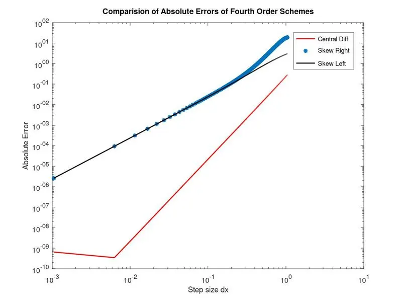
From the above plot it can be concluded that
For given dx values the central differencing scheme provides best result as it has the minimum error than all other schemes.
Increasing the step size dx, increases the error in all schemes. So the appropriate dx value should be choosen which is not having larger value in order to obtain best results in the schemes used.
Skewed right and skewed left schemes has errors that are almost equal below a certain range of value. But in compared to central differencing scheme, these two provide more error so we can say that central differencing with appropriate dx value should be used to get the solution closer to the second order derivative of a function.
But the central differencing in fourth order always requires the symmetric distribution of points around any node. That is always two nodes each should be present at any node we are to employ this scheme. But at the boundaries, this is quite not possible as nodes will not be there on either sides. So at these locations Skewed schems proves to be effective.
So skewed schemes can be employed where the distribution of nodes are not symmetric and also at boundaries, right and left skewed schemes are employed which gives the required solution.