Week 8 - Simulation of a backward facing step in OpenFOAM
Aim:
To simulate an incompressible-laminar-viscous flow through the backward facing step geometry.
Compare 2 case studies given and compare their results.
1.Simulate the flow without using any grading factor (i.e., GF = 1)
2. Simulate the flow with grading factor of 0.2. The cells should be finer near the walls (includig the step wall).
Theory
Backward Facing Step is widely known for its application in the studies on internal flows. The flow separation occurs in backward facing steps which is caused due to the sudden changes in the geometry. Due to this a zone of re-circulation is created, followed by a point of flow reattachment at the point where there is change in geometry. For our case we are tryin to simulate the incompressible-laminar-viscous flow meaning the fluid has viscosity, it is incompressible(density doesn't change) and flow is having low Reynold's number(doesn't have turbulance) so it is laminar.
To simulate we need a geometry, mesh specifications, initial and boundary conditions, processing the simulationa and verifying and studying the result in post processor.
The geometry of the Backward facing mesh is created using openFOAM software and its specifications are given below.
The domain specifications are provided in the following figure.
In openFOAM, we represent the geomerty as a set of blocks. So we divide the above geometry into five blocks as blocks can be create easily in openFOAM. To create a block 8 vertices are required and these vertices are numbered and shown below.
Using these vertices, the geometry is divided into five blocks.
Mesh specification for Geometry
- Number of cells along the x direction (longer dimension) = 200
- Number of cells along the longer y direction = 20;
To achieve the above requirements we navigate to a required folder in openFOAM tutorials and there we change the geometry, mesh specification, initial conditions as per our requirements in the exact files of the tutorials. Lets look at the way to navigate to the required tutorial folder to simulate the backward facing step.
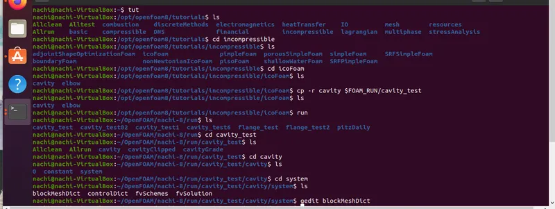
First we go to the inbuilt tutorials in openFOAM using the 'tut' command.
Requirement for our current simulation(Incompreesible flow) is in the incompressible folder. So we navigate to that folder by changing the directory to incompressible(cd command is used for it which means change directory).
In incompressible we use icoFoam solver for our simulation, so move to icoFoam folder. We can see the list of folders inside a folder by typing ls meaning list.
There we copy the 'cavity' folder in icoFoam to the seperate run folder($FOAM_RUN) using cp -r meaning to copy recurrsively as cavity folder will contain other folders. The simulation should always be ran after we copy the tutorials to run folder otherwise it'll affect the inbuilt tutorial.
Next we open our $FOAM_RUN folder(run is short-cut for it) and there we go to required cavity folder(here it is named as cavity_test).
There we go to cavity file and we can see 0, constant and system folders which contain details of initial conditions, information about constants and info about solvers respectively. We now navigate to system folder and there we create our required geometry in blockMeshDict and mesh for geometry is created.
blockMeshDict
The vertices of the geometry are specified first. The geometry is edited in the inbuilt folder by using gedit blockMeshDict as this file contains the information about vertices, how the blocks are created etc.
Geometry has 22 vertices and these are numbered from 0 to 21. The x, y and z co-ordinates are mentioned for each vertices.
Then geometry is divided into 5 blocks and each block is made of 8 vertices. Each block are created such a way that
First two vertices define the local x-axis, 2nd and 3rd verices define local y-axis and the fourth vertice is defined such a way that theplane created by four vertices is perpendicular to xy plane and pointing outwards. Next 4 vertices are defined in same order at some distance along z axis. So the same procedure is followed to create 5 blocks and hex command is used for creating this which means hexahedral mesh is created on the block.
After the block, number of cells along x, y and z axis are specified in a bracket. If it is (80 5 1) means 80, 5 and 1 cells are formed along local x, y and z axis. All dimensions are in mm as we have multiplied 1e-3 converting factor for inbuilt meters.
The grading for mesh is given in the preceding braces. Grading factor is the ratio of size of end cell to the size of starting cell. So our blocks should be defined perfectly otherwise it'll lead to a error meshing.
We are supposed to create a mesh such that it should be finer at the fixed boundaries and near step wall. So grading factor of 0.2 is used for our geometry. simpleGrading(0.2 5 1) means the size of the end cell is 0.2 times size of the starting cell along local x-axis in 1st block thus making the cells finer at the step wall. 5 means the sixe of end cell is 5 times the size of starting cell along y-axis making the below boundary finer in 1st block. The same way grading factor is used for other 4 blocks so the mesh is finer at required boundaries and step wall.
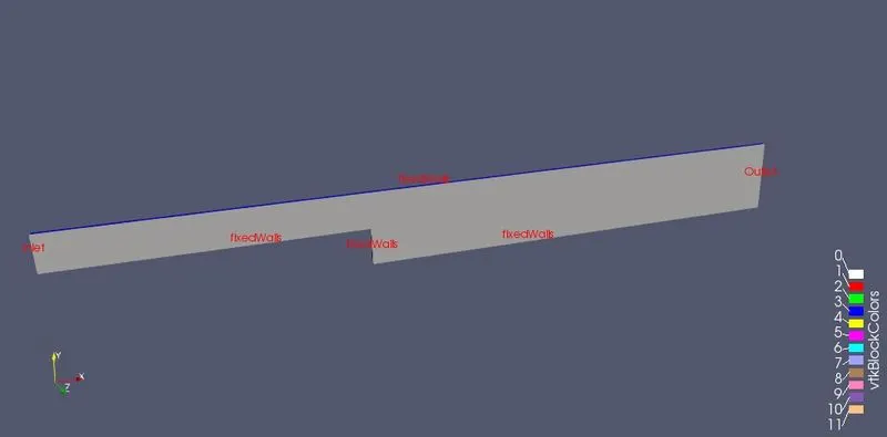
Next the Inlet and outlets of the geometry are created using patch type wall to required faces, fixed walls are specified and front and back faces in z axis are given 'empty' type wall. When the faces are viewed from outside, those faces need to specified in counter clockwise direction and specified in clockwise direction when viewed from inside the geometry such that the normal to the face points outwards.
By specifying all these correctly, our geometry is finished with the mesh specified, with fixed wall boundaries, Inlet and Outlet. Now our blockMeshDict file is set up as per requirement. Then blockMesh command is run which creates the mesh and specifies errors if any.
blockMeshDict file
/*--------------------------------*- C++ -*----------------------------------*\
  =========                 |
  \\      /  F ield         | OpenFOAM: The Open Source CFD Toolbox
   \\    /   O peration     | Website:  https://openfoam.org
    \\  /    A nd           | Version:  8
     \\/     M anipulation  |
\*---------------------------------------------------------------------------*/
FoamFile
{
    version     2.0;
    format      ascii;
    class       dictionary;
    object      blockMeshDict;
}
// * * * * * * * * * * * * * * * * * * * * * * * * * * * * * * * * * * * * * //

convertToMeters 1e-3;

vertices         //Vortex index
(
    (0 0 0)      //0
    (80 0 0)     //1
    (80 5 0)     //2
    (0 5 0)      //3
    (80 10 0)    //4
    (0 10 0)     //5
    (200 10 0)   //6
    (200 5 0)    //7
    (200 0 0)    //8
    (200 -10 0)  //9
    (80 -10 0)   //10
    (0 0 1)      //11
    (80 0 1)     //12
    (80 5 1)     //13
    (0 5 1)      //14
    (80 10 1)    //15
    (0 10 1)     //16
    (200 10 1)   //17
    (200 5 1)    //18
    (200 0 1)    //19
    (200 -10 1)  //20
    (80 -10 1)   //21
);

blocks
(
    hex (0 1 2 3 11 12 13 14) (80 5 1) simpleGrading (0.2 5 1)
    hex (3 2 4 5 14 13 15 16) (80 5 1) simpleGrading (0.2 0.2 1)
    hex (2 7 6 4 13 18 17 15) (120 5 1) simpleGrading (5 0.2 1)
    hex (1 8 7 2 12 19 18 13) (120 5 1) simpleGrading (5 5 1)
    hex (10 9 8 1 21 20 19 12) (120 10 1) simpleGrading (5 5 1)
);

edges
(
);

boundary
(
    Inlet
    {
        type patch;
        faces
        (
            (0 11 14 3)
            (3 14 16 5)
        );
    }

    Outlet
    {
        type patch;
        faces
        (
            (19 20 9 8)
            (18 19 8 7)
            (17 18 7 6)
        );
    }


    fixedWalls
    {
        type wall;
        faces
        (
            (4 5 16 15)
            (6 4 15 17)
            (20 21 10 9)
            (12 11 0 1)
            (1 10 21 12)
        );
    }


    frontAndBack
    {
        type empty;
        faces
        (
            (13 15 16 14)
            (12 13 14 11)
            (17 15 13 18)
            (18 13 12 19)
            (19 12 21 20)
            (0 3 2 1)
            (3 5 4 2)
            (2 4 6 7)
            (1 2 7 8)
            (10 1 8 9)
        );
    }
);

mergePatchPairs
(
)
;
// ************************************************************************* //
Case 1: The uniform mesh is created for the geometry using the grading factor (1 1 1) so the size of cells is uniform throughout the axes.
Case 2: The grading factor is given as mentioned above so geometry has Grading factor of 0.2 and is finer at boundaries and step wall and the remaining values will be same as case 1.
The geometry with boundaries is shown below
controlDict
In the same system folder we can see the controlDict file which can be used to change the simulation time settings.
The time step dt is taken such that the Courant number is below 1 so we get the stable and converging results. If this courant number is above 1, simulation may not converge.
Simulation is ran for 0.2 seconds which is mentioned in endTime with time step dt=0.0001.
We have CFL = nu * (dt/dx^2) where nu is kinematic viscosity and is equal to 0.01 m^2/s which is defined in the transportProperties file in the constant folder.
So the cobtrolDict file is set up as shown below.
/*--------------------------------*- C++ -*----------------------------------*\
  =========                 |
  \\      /  F ield         | OpenFOAM: The Open Source CFD Toolbox
   \\    /   O peration     | Website:  https://openfoam.org
    \\  /    A nd           | Version:  8
     \\/     M anipulation  |
\*---------------------------------------------------------------------------*/
FoamFile
{
    version     2.0;
    format      ascii;
    class       dictionary;
    location    "system";
    object      controlDict;
}
// * * * * * * * * * * * * * * * * * * * * * * * * * * * * * * * * * * * * * //

application     icoFoam;

startFrom       startTime;

startTime       0;

stopAt          endTime;

endTime         0.2;

deltaT          0.0001;

writeControl    timeStep;

writeInterval   100;

purgeWrite      0;

writeFormat     ascii;

writePrecision  6;

writeCompression off;

timeFormat      general;

timePrecision   6;

runTimeModifiable true;


// ************************************************************************* //
fvSchemes and fvSolution folders are shown below which contain the information of the various schemes used to solve the simulation, and the information of solvers, tolerance information etc. Solver her used is PCG(Preconditioned Conjugate Gradient) which accelerates the rate of convergence.
fvSchemes
/*--------------------------------*- C++ -*----------------------------------*\
  =========                 |
  \\      /  F ield         | OpenFOAM: The Open Source CFD Toolbox
   \\    /   O peration     | Website:  https://openfoam.org
    \\  /    A nd           | Version:  8
     \\/     M anipulation  |
\*---------------------------------------------------------------------------*/
FoamFile
{
    version     2.0;
    format      ascii;
    class       dictionary;
    location    "system";
    object      fvSchemes;
}
// * * * * * * * * * * * * * * * * * * * * * * * * * * * * * * * * * * * * * //

ddtSchemes
{
    default         Euler;
}

gradSchemes
{
    default         Gauss linear;
    grad(p)         Gauss linear;
}

divSchemes
{
    default         none;
    div(phi,U)      Gauss linear;
}

laplacianSchemes
{
    default         Gauss linear orthogonal;
}

interpolationSchemes
{
    default         linear;
}

snGradSchemes
{
    default         orthogonal;
}


// ************************************************************************* //
fvSolution
/*--------------------------------*- C++ -*----------------------------------*\
  =========                 |
  \\      /  F ield         | OpenFOAM: The Open Source CFD Toolbox
   \\    /   O peration     | Website:  https://openfoam.org
    \\  /    A nd           | Version:  8
     \\/     M anipulation  |
\*---------------------------------------------------------------------------*/
FoamFile
{
    version     2.0;
    format      ascii;
    class       dictionary;
    location    "system";
    object      fvSolution;
}
// * * * * * * * * * * * * * * * * * * * * * * * * * * * * * * * * * * * * * //

solvers
{
    p
    {
        solver          PCG;
        preconditioner  DIC;
        tolerance       1e-06;
        relTol          0.05;
    }

    pFinal
    {
        $p;
        relTol          0;
    }

    U
    {
        solver          smoothSolver;
        smoother        symGaussSeidel;
        tolerance       1e-05;
        relTol          0;
    }
}

PISO
{
    nCorrectors     2;
    nNonOrthogonalCorrectors 0;
    pRefCell        0;
    pRefValue       0;
}


// ************************************************************************* //
Initial Conditions:
The initial conditions can be provided in the '0' folder which has the information of pressure and velocity at the 0 time means at the start of the simulation(Initial condition).
using gedit U and gedit p command, Initial velocity and pressure can be set up as per our requirement.
Velocity Inlet(U)
The initial velocity is specified at the inlet of the geometry and is kept uniform or constant at inlet with 1m/s along x-axis and 0 along remaining axes.
At all other walls it is taken as 0. No slip condition is given at fixed walls meaning there is no relative movement between the boundary and the fluid layer, and for front and back faces are made as empty type walls.
/*--------------------------------*- C++ -*----------------------------------*\
  =========                 |
  \\      /  F ield         | OpenFOAM: The Open Source CFD Toolbox
   \\    /   O peration     | Website:  https://openfoam.org
    \\  /    A nd           | Version:  8
     \\/     M anipulation  |
\*---------------------------------------------------------------------------*/
FoamFile
{
    version     2.0;
    format      ascii;
    class       volVectorField;
    object      U;
}
// * * * * * * * * * * * * * * * * * * * * * * * * * * * * * * * * * * * * * //

dimensions      [0 1 -1 0 0 0 0];

internalField   uniform (0 0 0);

boundaryField
{
    Inlet
    {
        type            fixedValue;
        value           uniform (1 0 0);
    }

    Outlet
    {
        type            zeroGradient;
    }


    fixedWalls
    {
        type            noSlip;
    }

    frontAndBack
    {
        type            empty;
    }
}

// ************************************************************************* //
Pressure Outlet(p)
The initial pressure is specified at the outlet of the geometry with the constant value 0.
/*--------------------------------*- C++ -*----------------------------------*\
  =========                 |
  \\      /  F ield         | OpenFOAM: The Open Source CFD Toolbox
   \\    /   O peration     | Website:  https://openfoam.org
    \\  /    A nd           | Version:  8
     \\/     M anipulation  |
\*---------------------------------------------------------------------------*/
FoamFile
{
    version     2.0;
    format      ascii;
    class       volScalarField;
    object      p;
}
// * * * * * * * * * * * * * * * * * * * * * * * * * * * * * * * * * * * * * //

dimensions      [0 2 -2 0 0 0 0];

internalField   uniform 0;

boundaryField
{
    Inlet
    {
        type            zeroGradient;
    }

    Outlet
    {
        type            fixedValue;
        value           uniform 0;
    }


    fixedWalls
    {
        type            zeroGradient;
    }

    frontAndBack
    {
        type            empty;
    }
}

// ************************************************************************* //
Now all the required inputs are given and the mesh is verified using blockMesh command and the simulation is ran using 'icoFoam' command which is the solver in out case.
Result
Case 1: Grading Factor - 1
Mesh of the geometry
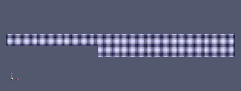
As the grading factor used is 1, we can see size of all the cells in the geometry are equal. The mesh can be further made finer by using more number of cells in a block, but more number of cells leads to increased simulation time.
Velocity Contour
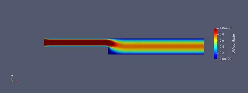
The velocity contour for grading factor 1 can be seen above. The velocity is which is specied as 1m/s at inlet, is higher before the flow reaches the step and as the fluid flow past the step wall, fluid expands and the velocity of the flow can be seen reducing at the centre of the geomtry. The velocity is further reduced at the boundaries or fixed walls. After the step wall velocity along y axis is constantly varying(is lesser compared to before) due the expansion in the flow when it reaches a larger area.
Pressure Contour
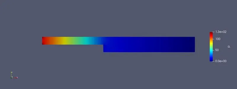
The pressure is made as zero at the outlet in our initial condition. So pressure can be seen at lower values at the outlet. Pressure is maximum at the inlet of the geometry and goes on reducing as the fluid flows towards the step. After the step wall, it can be seen that the pressure is reduced by larger amount.
Case 2: Grading Factor - 0.2
Mesh
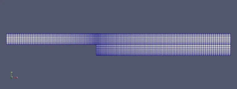
Due to the introduction of grading factor of 0.2, the size of the cells is not uniform in the geometry. It can be seen that the mesh is finer at the step wall and at the boundaries. At the step wall and boundaries there may be a chance of flow seperation and recirculation and re attachement of the flow due to the sudden change in the geometry. So the variables at these locations should be calculated we higher accuracy. So for that the mesh is need to made finer at walls and step face and this can be done by using grading factor. So this is the use of grading factor in any geometry which makes the mesh finer or coarser according to the requirement.
Velocity Contour
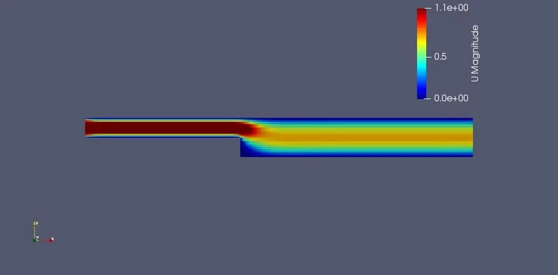
The flow properties of the velocity can doesn't change and is almost similar to the case of grading factor 1. Velocity reduces after the step wall due to the expansion and is higher at core compared to the boundaries past the step wall.
To exactly find out how velocity changes after step wall, the velocity along y-axis at any point after step wall(say 0.085m) need to be compared.
Pressure Contour
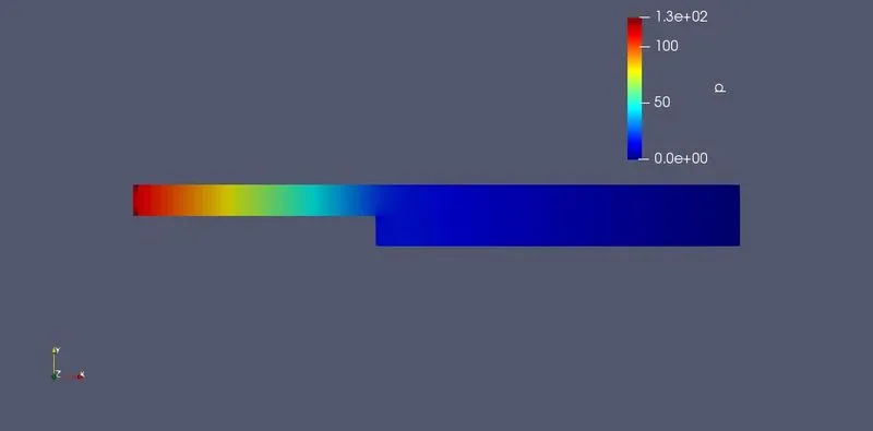
The properties of pressure in this case is also same as that for grading factor 1(there may be slight changes). The pressure is more before the step wall, higer at inlet and reduces as fluid flows along the geometry and comes lower value at the outlet.
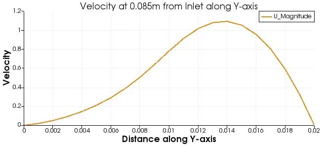
Velocity Plot at a distance 0.085m from Inlet for Grading Factor - 1
Velocity Plot at a distance 0.085m from Inlet for Grading Factor - 0.2
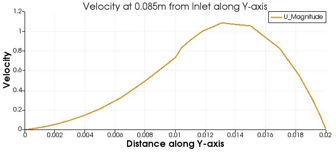
Finally the velocity at a distance of 0.085m from the inlet of the geometry along y-axis is plotted for two different cases of grading factor and compared. The graphs are plotted using plot over line command in the paraview post processor and the two points with x, y and z coordinates are specified to plot the graphs in the software.
When the grading factor is 1, we can see the smoother curve of velocity as compared to grading factor 0.2. This comes from the fact that the size of the cell along y-axis at a distance of 0.085m from inlet is not equal throughout and the size of cell in grading factor 0.2 is goes on increasing and decreasing from lower fixed wall to upper one.
It can be seen that the velocity is continuously changing along y axis at 0.085m from Inlet. This location is just after the step wall, so the fluid is expanding at this region and thus the velocity is continuously changing. The velocity is higher at the centre of the geometry and reduces on either side towards the fixed walls. The same can be seen from the plot. As the distance along y-axis is increases, the velocity increases and reaches its maximum value some where at the centre of the geometry(Near 0.013 from lower bounary along y axis) and further velocity decreases as it reaches boundary or fixed wall along y-axis.