Week 6.2 - Setting up a model (Hanging Node)

AIM

The objective of the project is to create thermal analysis of the hanging node model.

TASK

• Create non-conformal mesh assembly and use mesh separately option with slack values.
• Create the physics model for the hanging node and plot the results for the model.

Model

File --> unpack project --> hanging node.tzr - This opens the hanging node model and click on View --> default shading --> solid.

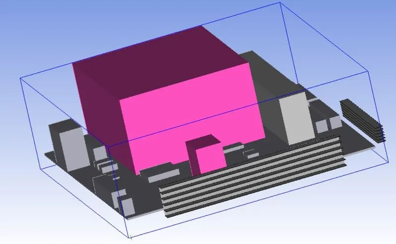
The mesh refinement around CAD objects need to be high inorder to capture the model accurately. Note that this mesh count results from using the non-conformal meshing technique, which reduces mesh bleeding and mesh count.

In order to capture the CAD model the mesh is too refined around the CAD objects where refinement of mesh causes increase in the simulation time. So Multi level meshing is used mesh elements reduction.

Different methods to improve mesh resolution

i) Multi level meshing

It enables local refinement from a starting Cartesian mesh generated using the max sizes you specified. Multi-level meshing is useful if you have a large variation of length scales in your model. The refinement can be controlled such that the initial mesh is refined in an area where the mesh needs to be finer in order to resolve some geometrical features or gaps. This will significantly reduce the overall mesh count while providing adequate mesh resolution where it is needed. Multilevel meshing applies to 2D and 3D cut cell as well as stair-stepped meshing.

• Max levels is the maximum number of levels that may be required to achieve the desired mesh refinement based upon curvature/proximity. For a given coarse mesh the desired proximity/curvature based refinement may be achieved even before reaching the max levels.

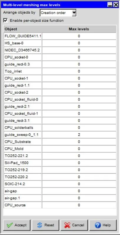
• Edit levels enables you to specify refinement levels for selected objects. Per-object meshing levels can be used in conjunction with the max level and size functions.

When Enable per-object size function is enabled, the size functions (proximity and/or curvature) are used to subdivide the mesh around the object up to the max level specified for the object. When Enable per-object size function is disabled, the mesh is subdivided to the max-level everywhere on the object.

The objects around the Fan guide are group to a individual assembly for the further reduction in the mesh elements.

ii) Mesh assemblies separately

It indicates whether or not ANSYS Icepak should generate a non-conformal mesh for the assemblies that have the Mesh separately option turned on. This option enables you to turn off (or on) all defined non-conformal meshing for the entire model.

The separate assembly for the objects around the Fan guide are created.

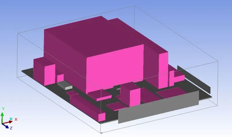
Sheet metal HS assy

The Mesh sepaartely option is selected for this assembly and the folowing data are provided.

i) Slack setting

Min X - 2 mm.

Max X - 2 mm.

Min Y - 2 mm.

Max Y - 2 mm.

Min Z - 2mm.

Max Z - 2mm.

ii) Mesh type

Max element size X - 1 mm.

Max element size Y - 0.5 mm.

Max element size Z - 1 mm.

Min Gap X - 0.06 mm.

Min Gap Y - 0.06 mm.

Min Gap Z - 0.06 mm.

The Multi level mesh option is selected and max levels is set to 2 and under options set unifrom mesh parameters is selected & use average is selected.

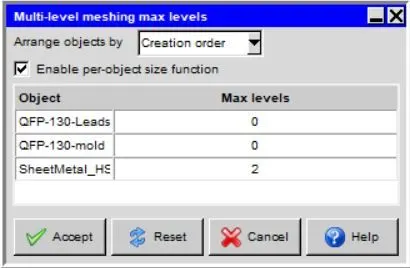
Fan guide

The Mesh sepaartely option is selected for this assembly and the folowing data are provided.

i) Slack setting

Min X - 2 mm.

Max X - 2 mm.

Min Y - 2 mm.

Max Y - 0.

Min Z - 2 mm.

Max Z - 3 mm.

ii) Mesh type

Max element size X - 5 mm.

Max element size Y - 2 mm.

Max element size Z - 4 mm.

Min Gap X - 0.01 mm.

Min Gap Y - 0.01 mm.

Min Gap Z - 0.01 mm.

The Multi level mesh option is selected and max levels is set to 2 and under options set unifrom mesh parameters is selected & use average is selected.

Mesh Settings

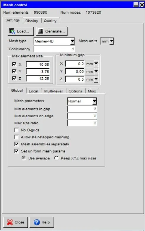
All the paarmeters are kept unchanged and the model is meshed by clicking on generate option.

Mesh type - Mesher-HD.

Concurrency - 1.

Max element size

Max element size X - 10.65 mm.

Max element size Y - 3.75 mm.

Max element size Z - 12.25 mm.

Minimum gap

Min Gap X - 0.2 mm.

Min Gap Y - 0.06 mm.

Min Gap Z - 0.5 mm.

Global

Mesh paarmeters - Normal.

Min elements in gap - 3.

Min elements on edge - 2.

Max size ratio - 2.

Select the set uniform mesh parameters and choose use average method.

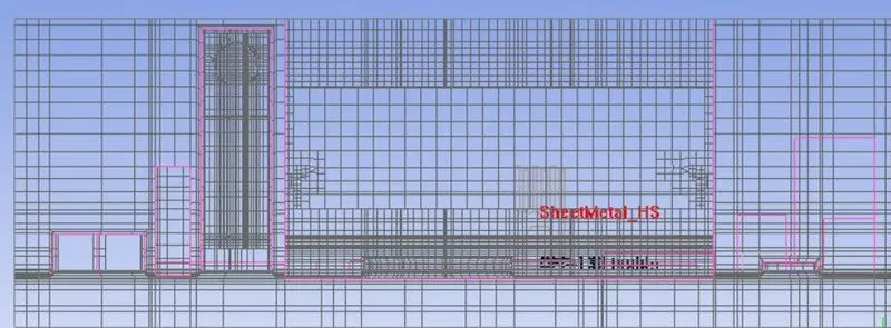
The mesh refinement has captured the CAD model more accurately. The Cut plane of the model around the CAD objects is provided below.

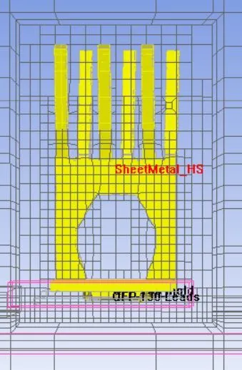
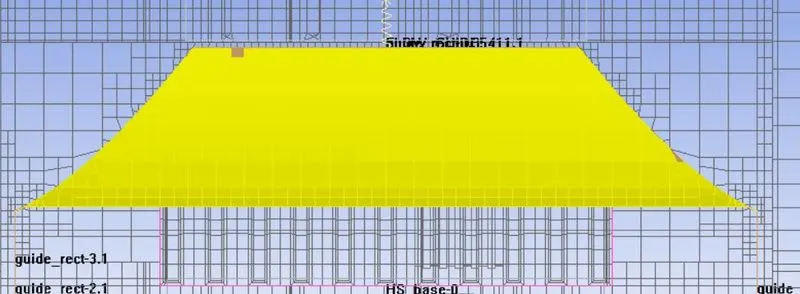
Mesh along X plane

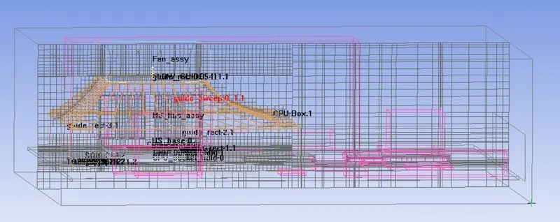
Mesh along Y plane

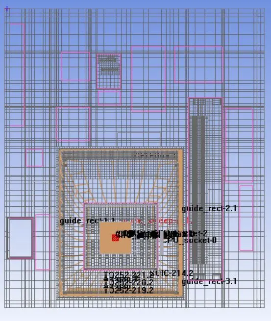
Mesh along Z plane

Mesh Verification

Face alignment

• It is the measure of mesh quality defined by face alignment index = C0C1.f
• C0 & C1 are the centroids of two adjacent elements are normal vector to the face between the two elements.
• Range of face alignment 0 (bad) to 1 (good) & value greater than 0.05 (preferred) & value greater than 0.15 provide better results.

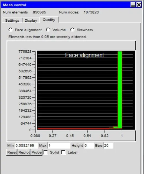
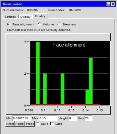
The min value of the model is 0.0882 and in order to get better results minvalue must be greater than 0.15 & in our model the 13 elements were under 0.15 value. The model is good for the analysis.

Volume

• Preferable volume of mesh to be greater than 1e-13 for single precision solver & greater than 1e-15 for double precision.
• Max / Min cell volume should be less than 10^7 for single precision & must be less than 10^12 for double precicion since very small volume create divergence of the solution.

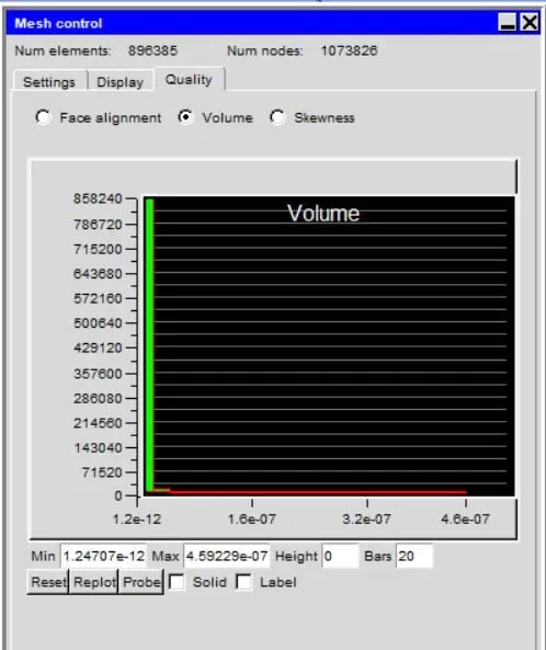
The volume of the mesh greater than 10^-13 & Max / Min cell ratio is around 350000 which is in required range & the single precision is used for this model.

Skewness

It determines how close to the ideal & based on the equilateral volume. The value greater than 0.2 provide fair cell quality.

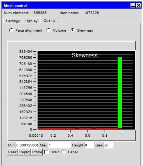
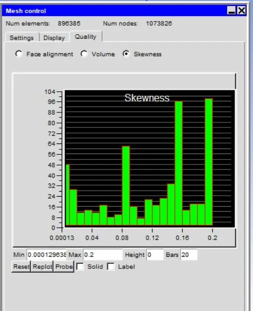
The min value of the skewness is 0.005 and the quality below 0.25 have around 1000 elements this is due to the sharp curves around the guide sweep and sheet metal HS and max multi level mesh is kept at 2 but further refinement will reduce the skewed elements around the corner of the objects.

Solver

The three dimensional steady state Navier stokes equations for the model are solved within the computational domain.

General Setup

• Variables solved - flow and temperature.
• Radiation - Off.
• Flow regime - Turbulent - The zero equation are solved for the turbulent model.

The natural convection are not consider for this model & also gravity vector are not consider.

The defaults value of the parameters are set to default.

Transient Setup

• Time variation - Steady

Solution Initialization

X velocity - 0.

Y velocity - 0.

Z velocity -0.

Temperature - ambient.

Basic settings

No of iterations - 100.

Convergence criteria

Flow - 0.001.

Energy - 1e-10.

Joule heating - 1e-7.

Parallel Settings

Configuration - parallel.

Parallel options - 4 processors.

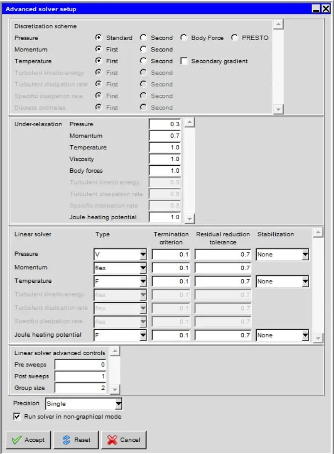
Advance Solver Setup

Results

The residuals for the following equations are plotted against the number of iterations:

• Continuity equation.
• X-momentum equation.
• Y-momentum equation.
• Z-momentum equation.
• Energy equation.

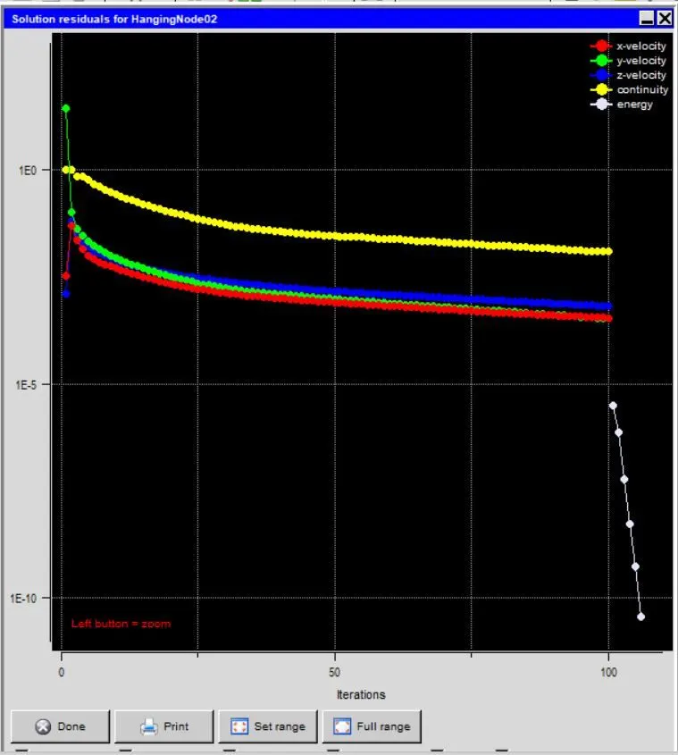
The solution is run for 100 iterations and the contiuity and momentum has converged for the solution.

Plot

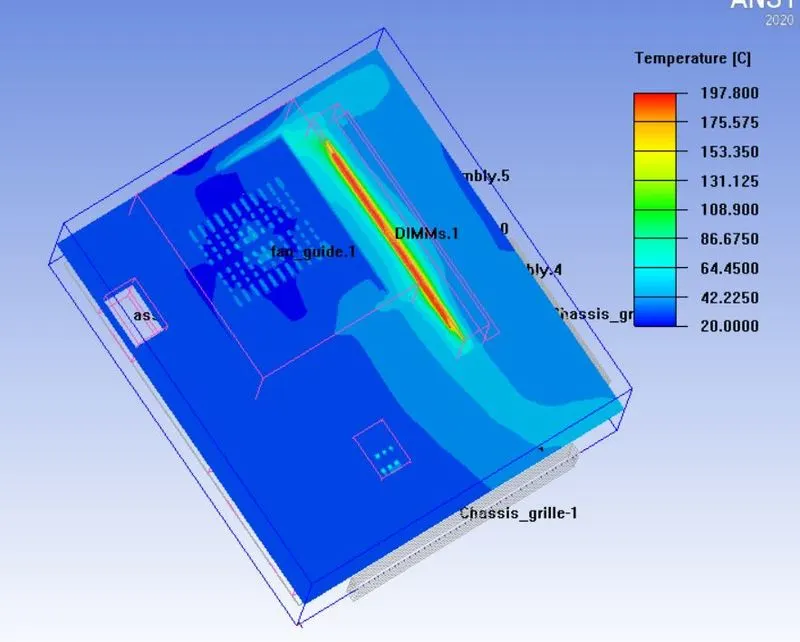
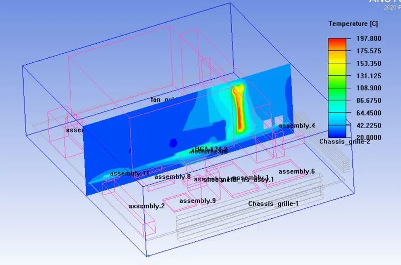
Temperature Contour

Y cut plane

Z cut plane

Model Temperature plot

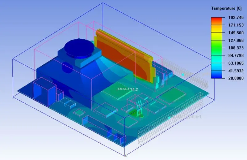
The maximum temperature within the computational domain is 192.75 degC. The hotter objects in the model interacts with the objects due to the heat transfer from them and the temperature of the objects increases. The temperature at the other end of the model is at the ambient condition.

Velocity Contour

X cut plane

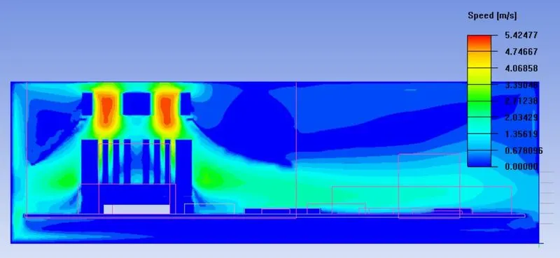
Y cut plane

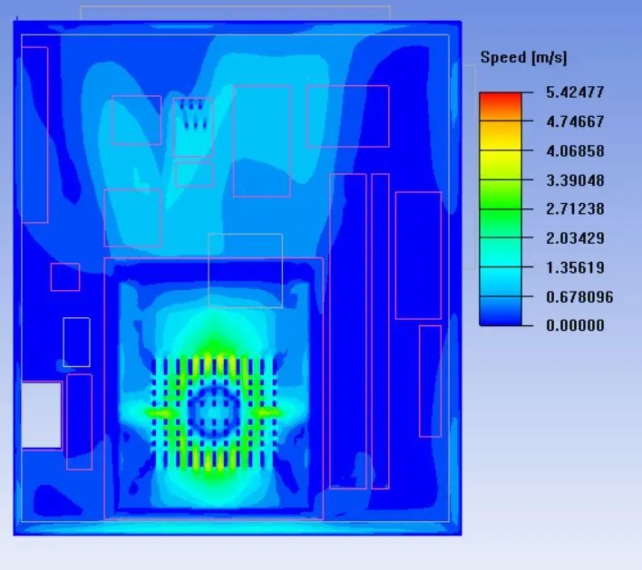
The contour plot of the velocity is highest around the fan at which the velocity is around 5.3 m/s. The air leaves through the assembly through the grilles.

Contour plot

X cut plane

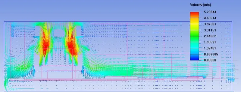
The vector plots for the velocity for the air at 1000 points distributed uniformly through the X plane. The vectors the air achieves maximum velocity as it passes through the fan. The velocity vector are able to capture the recirculation zones established on the X plane.

Conclusion

In this project the given model of the electronic enclosure was meshed using ANSYS Icepak using the non-conformal meshing, per-object meshing parameters and multi-level meshing. The three dimensional steady-state governing equations for the model were solved for flow and temperature within the computational domain in the Icepak.

• The maximum temperature within the computational domain is 192.75 deg.C.
• The maximum air velocity within the computational domain is 5.298 m/s.