Week 11 - Louver/Grille characterization

Aim

The objective of the project is to simulate a hexa grille placed at the center of the channel for a streamline flow and do a parametric optiization of the design.

Task

• Define a parameter to optimize the design.
• Define trials.
• Define primary and compound functions that you want to report.
• Calculate parametric solutions.
• Report and plot parametric results.

Geometry

Cabinet : It creates a fluid region around the model for which the governing equations are solved.

i) Geometry 

Shape - Prism.

Specified By - Start/end.

Start Xs - 0 mm. 

Start Ys - 0 mm.

Start Zs - -80 mm.

End Xe - 12.7 mm.

End Ye - 7.363 mm.

End Ze - 80 mm.

ii) Properties - The wall type for the cabinet is defined.

Min X - Wall.

Max X - Wall.

Min Y - Wall.

Max Y - Wall.

Min Z - Opening.

Max Z - Opening.

Reynolds Number:

Re = u*L/v = rho*u*L/mu

where:

rho - Density of the fluid (kg/m3)

u - flow speed (m/s)

L - Characteristic linear dimension (m)

mu - dynamic viscocity of fluid (N-s/m2)

v - kinematic viscocity of fluid (m2/s)

L = 4*A/P

   = 4 * (12.7*7.363)*1e-6/(2*(12.7+7.363)*1e-3)

   = 0.009321647 m.

V = Re*v/L

    = $Re * 1.84e-5 / 9.322e-3 and define this as z-velocity for the Min Z opening.

Block

i) Geometry 

Shape - Polygon.

Specified By - Start/end.

Plane - X-Y.

Height - 1mm.

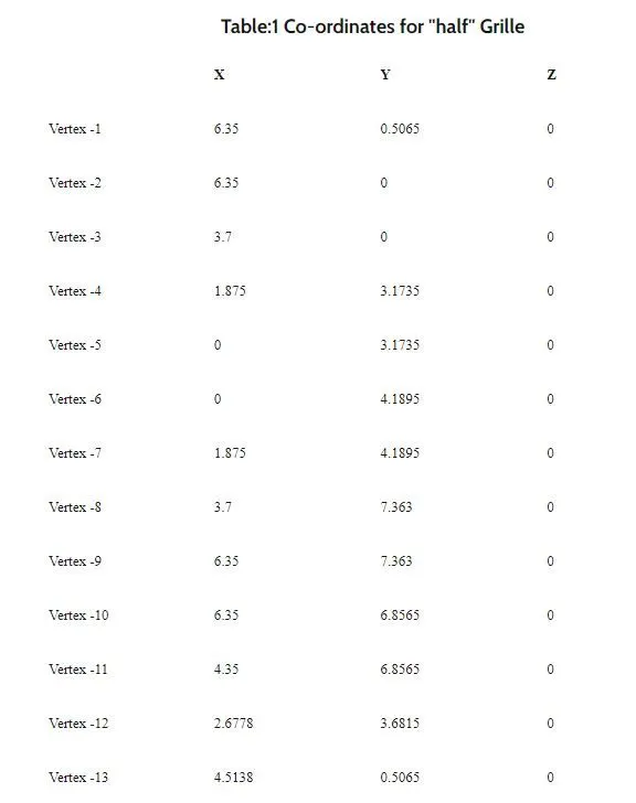
Mirror the object about the high end and choose the plane as X-Y.

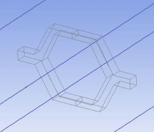
Assemble

Select all the blocks and click on create --> assembly.

Under the meshing tab choose Mesh separately,

i) Slack setting

Min X - 0 mm.

Max X - 0 mm.

Min Y - 0 mm.

Max Y - 0 mm.

Min Z -  5 mm.

Max Z - 5 mm.

Mesh control

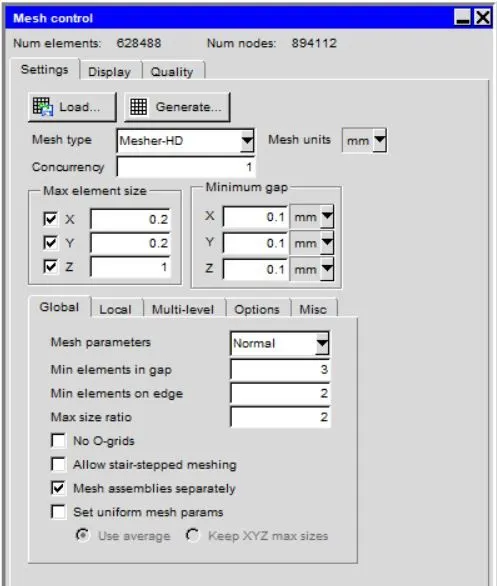
Mesh along Y plane

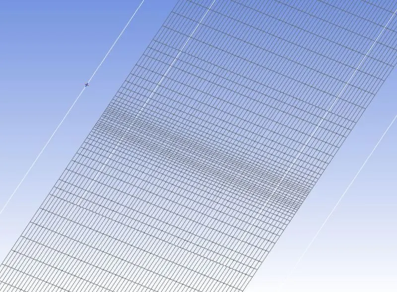
Mesh along Z plane

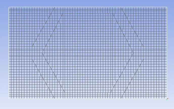
Mesh Verification

Face alignment

• It is the measure of mesh quality defined by face alignment index = C0C1.f
• C0 & C1 are the centroids of two adjacent elements are normal vector to the face between the two elements.
• Range of face alignment 0 (bad) to 1 (good) & value greater than 0.1 (preferred) & value greater than 0.15 provide better results.

         

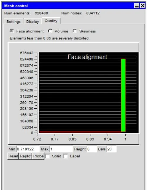
The min value of the model is 0.718 which is ideal for the results.

Volume

• Preferable volume of mesh to be greater than 1e-13 for single precision solver & greater than 1e-15 for double precision.
• Max / Min cell volume should be less than 10^7 for single precision & must be less than 10^12 for double precicion since very small volume create divergence of the solution.

        

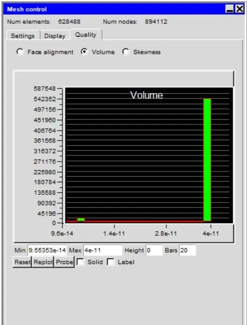
The volume of the mesh greater than 10^-14 & Max / Min cell ratio is around 420 which is in required range & the single precision can be used for this model. 

Skewness

It determines how close to the ideal & based on the equilateral volume. The value greater than 0.5 provide good cell quality.

        

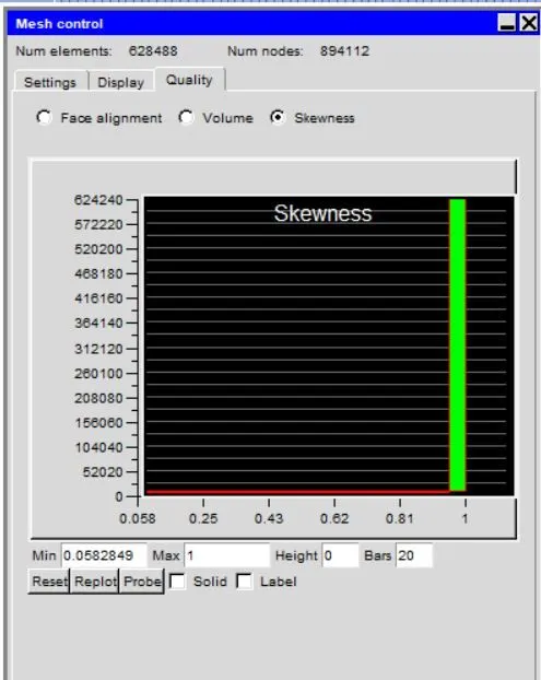
The min value of the skewness is 0.058.

In parameter and optimization select the parametric trails and the discrete values are set to 10 50 100 500 1000 2000 3000 4000.

Report --> Summary report and create four objects.

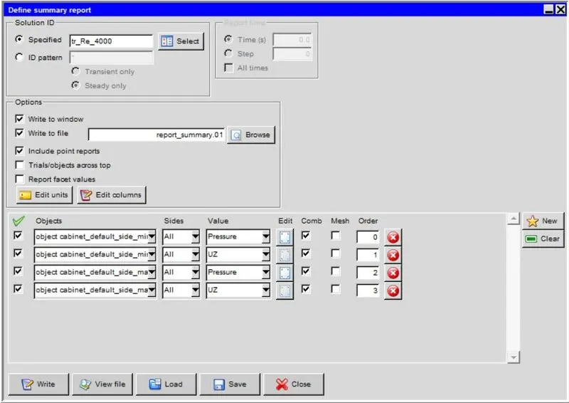
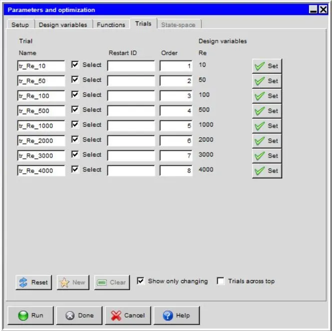
To create primary functions, click on the new under primary functions tab

i) Function name - Pstat_out.

Function type - Report Summary.

Item - Cabinet_default_side_maxz_pressure and choose Max.

ii) Function name - Vel_out.

Function type - Report Summary.

Item - Cabinet_default_side_maxz_Uz and choose Mean. 

iii) Function name - Pstat_in.

Function type - Report Summary.

Item - Cabinet_default_side_minz_pressure and choose Max. 

iv) Function name - Vel_in.

Function type - Report Summary.

Item - Cabinet_default_side_minz_pressure and choose Mean.

To create compound functions, click on the new under compound functions tab

i) Function name - Pdyn_in

   Definition - 0.5*1.16*$Vel_in*$Vel_in.

ii) Function name - Pdyn_out

   Definition - 0.5*1.16*$Vel_out*$Vel_out.

iii) Function name - Ptot_in

   Definition - $Pstat_in+$Pdyn_in.

iv) Function name - Ptot_out

   Definition - $Pstat_out+$Pdyn_out.

v) Function name - Kloss

   Definition - $Ptot_in - $Ptot_out / $Pdyn_out.

Numerical Setup

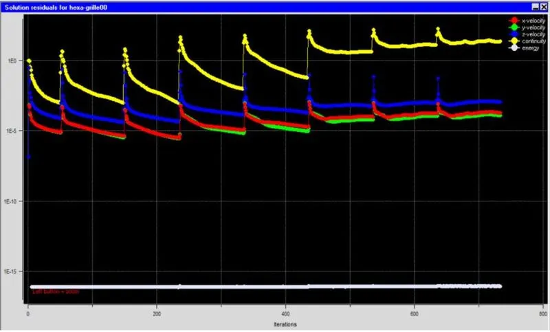
Report_Summary

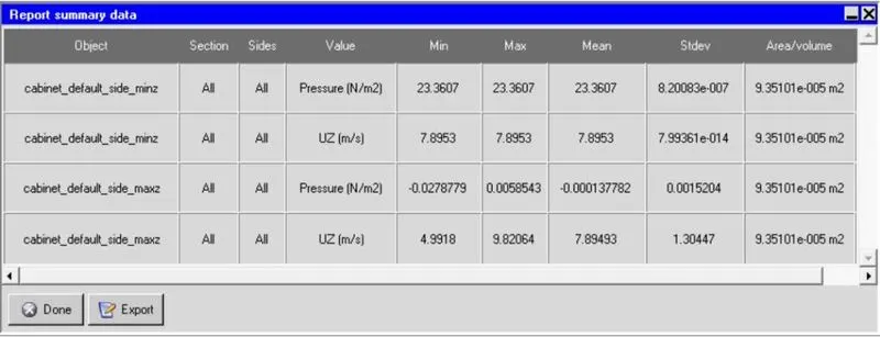
Parametric report

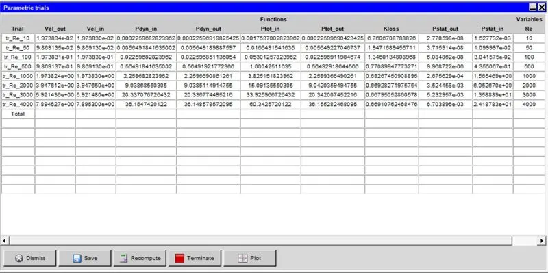tf

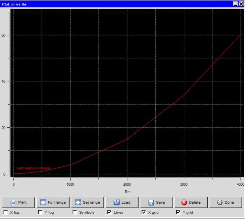
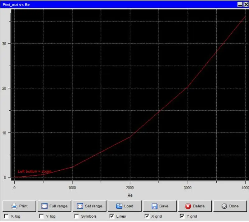
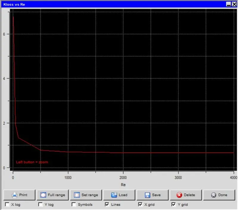
Graph plots

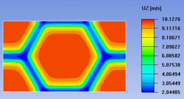
Velocity plot

Conclusion

In this project the given model of the grille is simulated using Ansys Icepak. The three dimensional steady-state governing equations for the model were solved for flow and temperature within the computational domain in the Icepak. The pressure at both inlet and outlet increases with the increase in the Reynolds number. The coefficient of the loss decreases and then becomes constant after 1000 reynolds number.

• The maximum air velocity within the computational domain is 10.13 m/s.