Week 4 - CHT Analysis on Exhaust port

CHT ANALYSIS ON EXHAUST PORT

Aim : Conduct CHT analysis on exhaust port in ANSYS Fluent

Objectives:

1. Description on why and where CHT is used
2. Maintain the y+ value according to the turbulence model and justify the results.
3. Calculate the wall/surface heat transfer coefficient on the internal solid surface and show the velocity and temperature in appropriate areas
4. Explanation on how to verify the CHT predictions are right
5. Factors on which the prediction depends on

Theory:

Exhaust port : These are thermal shafts or vents that are used to let the hot gases due to combustion out of the engines. Exhausts ports are used in industries for the same reason to let the hot gases escape.

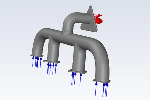
Conjugate Heat Transfer Analysis (CHT):

The Conjugate Heat Transfer (CHT) analysis type allows for the simulation of heat transfer between solid and fluid domains by exchanging thermal energy at the interfaces between them. conjugate heat transfer (CHT) analysis can accurately predict heat transfer by simultaneous solving all the relevant solid and flow field heat transfer processes,

Application:

1. The simulation of heat exchangers
2. Cooling of electronic equipment
3. General-purpose cooling and heating systems.
4. conduction through solids
5. Free and forced convection in the gases/fluids
6. Thermal radiation

Advantages:

The CHT approach has an advantage over FE thermal analyses in that wall heat transfer coefficients and their local variations on surfaces are directly calculated within the model rather than based on simplified empirical calculations. The CHT approach therefore has benefits for those applications where heat transfer is either non-uniform or difficult to calculate empirically.

Case setup:

Geometry:

• Extract the volume by selecting all the edges and name it as fluid body

Prepare > Volume extract > edge select

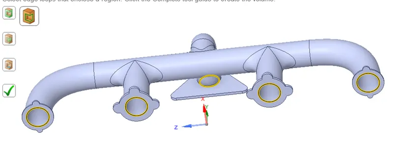
• Select the created fluid volume and solid volume and move them to new component

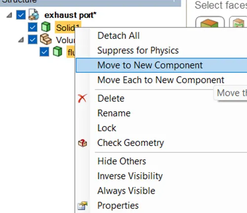
• Select the properties of the body and set topology to shar
• In workbench tool select share option.
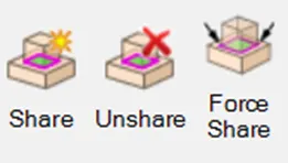
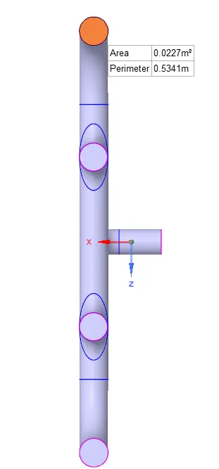
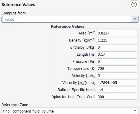
• Measure the inlet area and we use that area as refernce area for calculation of surface heat ransfer coefficient.

Meshing:

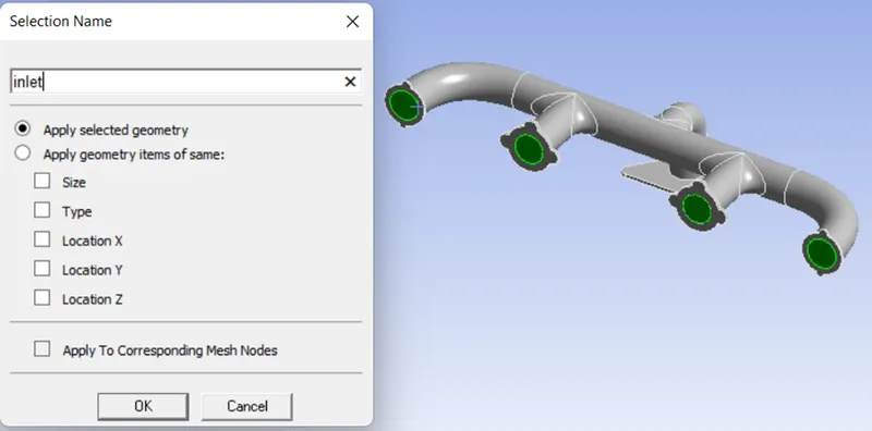
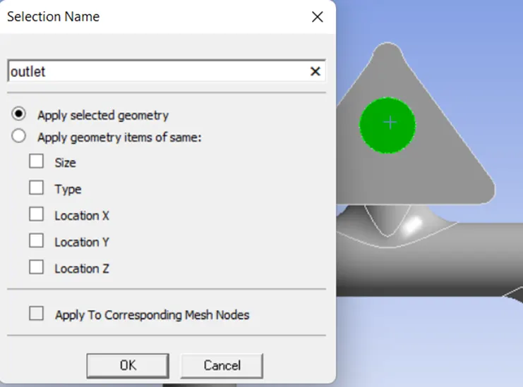
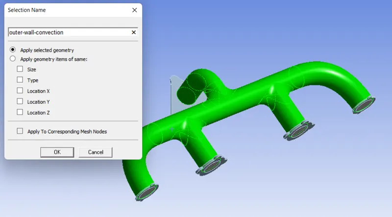
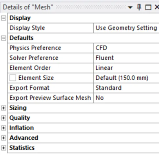
• Name inlet, outlet and outer convective wall.

• Create base mesh
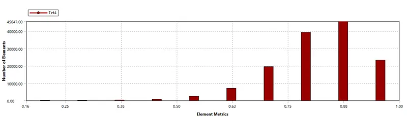
• Mesh quality:

• Base mesh:

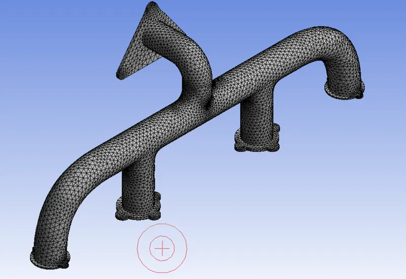
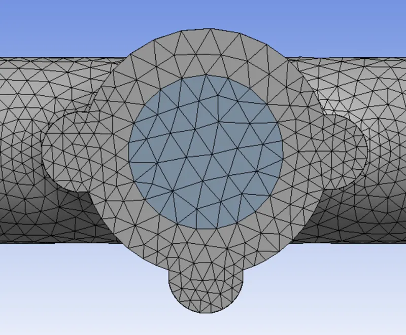
• Number of elements:

Setup:

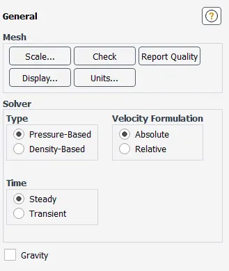
• Set Pressure based steady solver.

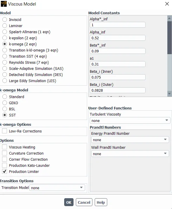
• Use k-omega SST turbulence model and check energy parameter.

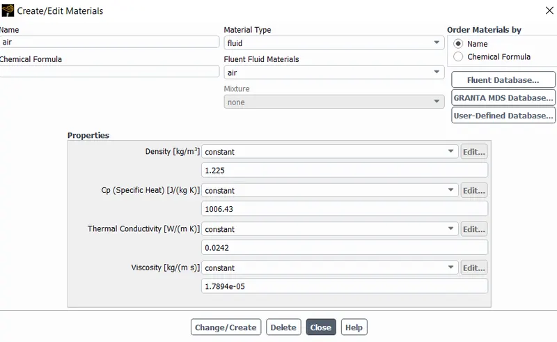
• Set fluid material as air and solid material as aluminum
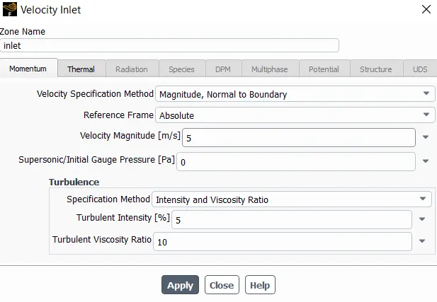
• Set boundary conditions at inlet, outer convection wall and outlet.
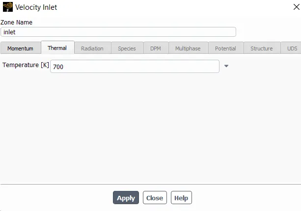
• Set inlet velocity 5m/s and temperature 700K
• 
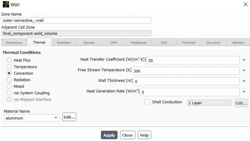
• Set heat transfer coefficient as 20 W/(m^2*K)
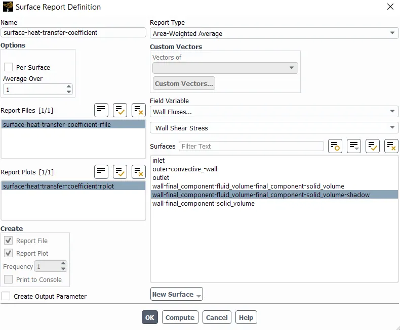
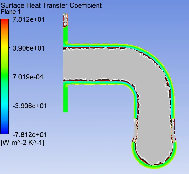
• Create report definition for surface heat transfer coefficient at interface, here there are two interfaces one on the fluid side and another on the solid side, shadow region indicates interface on the solid side, no matter what interface we select they both give same value for heat transfer coefficent but differ in sign as heat is being transfered from fluid to solid, fluid interface gives nagetive value where as solid solid interface gives positive value.
• 
• Set referance values of areq,temperature and velcoity.
• 
• Use SIMPLE solution method and first order upwind method for momentum as higher order schemes tend to be more unstable.
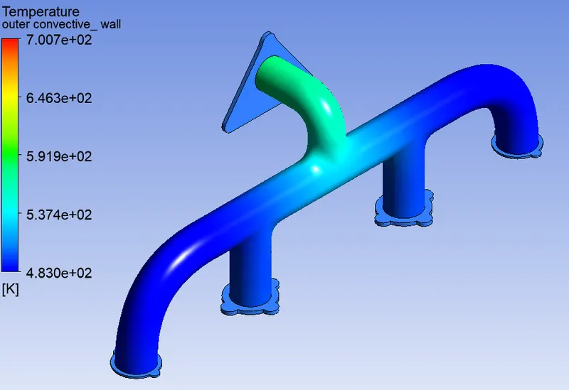
• Initialize the setup and create temperature contour.

Results:

Surface heat transfer coefficient plot:

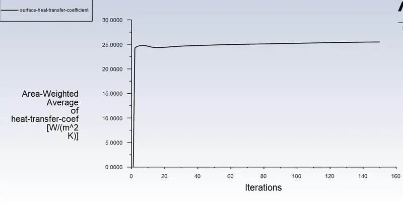
Heat transfer coefficient value at solid side interface:

Residuals:

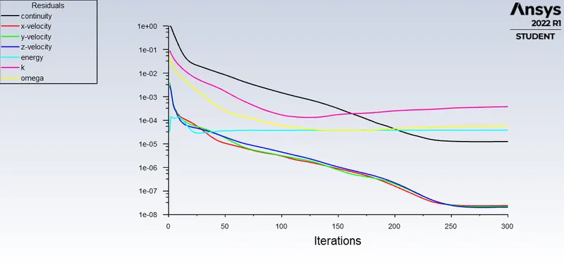
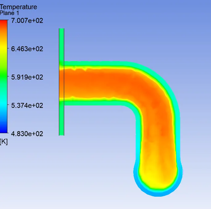
Temperature contour:

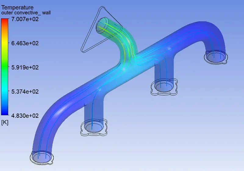
Velocity streamlines:

Temperature contour at outlet:

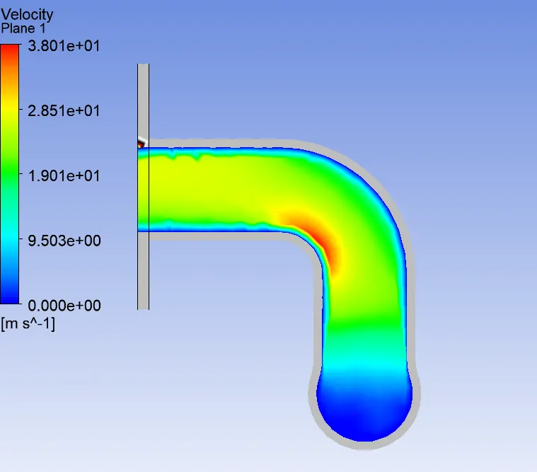
Velocity contour at outlet:

Surface heat transfer coefficient:

Refined mesh:

Meshing:

• Decrease the element size to 0.08m and provide inflation layers.
• Find wall sapcing for Y+ value of 1 and use it as a first layer thickness to create 10 inflation layers both on solid and fluid side.

Wall spacing calculations:

wall spacing(`Deltas`) = `(Y^+mu)/(U_(Fric)rho)`

where:

`U_(Fric) = sqrt(tau_(wall)/rho)`

`tau_(wall) = (C_(f)rhoU^2)/2`

`C_f = 0.026/(Re^(1/7))`

where:

`U =`Free stream velocity

`Re`= Reynolds number

`rho =` Density

`L=` Reference length

`tau_(Fric)`= Shear stress

`mu`= Dynamic viscocity

`C_f`= Skin friction coefficient

Given:

• velocity(U) = 5 m/s
• reference length (L) = diameter of inlet (d)
• d = 0.17 m
• `rho = 1.225 (kg)/(m^3)`
• dynamic viscocity(`mu`) = `0.000017894 (kg)/(ms)`
• y+ = 1

Calculations:

1. `Re = (rhoUL)/(mu)` = 58189.8960
2. `C_f = 0.026/(Re^(1/7)` = 0.00646
3. `tau_(wall) =``(C_(f)rhoU^2)/2`= 0.0989 `N/m^2`
4. `U_(Fric) = sqrt(tau_(wall)/rho)`= 0.2841 `m/s`

`Deltas = (Y^+mu)/(U_(Fric)rho)`= 0.00005610168684138391m

use this wall spacing value to create inflation layers

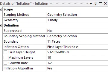
Mesh detail:

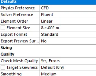
Number of elements:

Results:

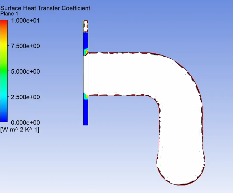
Surface heat transfer coefficient plot:

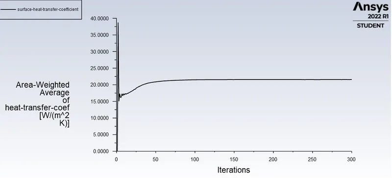
Heat transfer coefficient value at solid side interface:

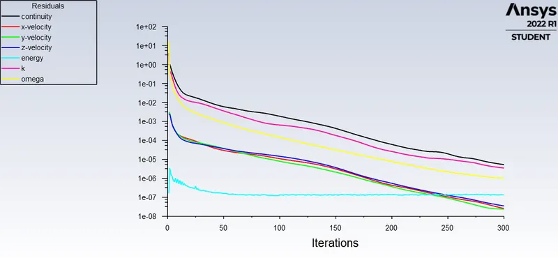
Residuals:

Temperature contour:

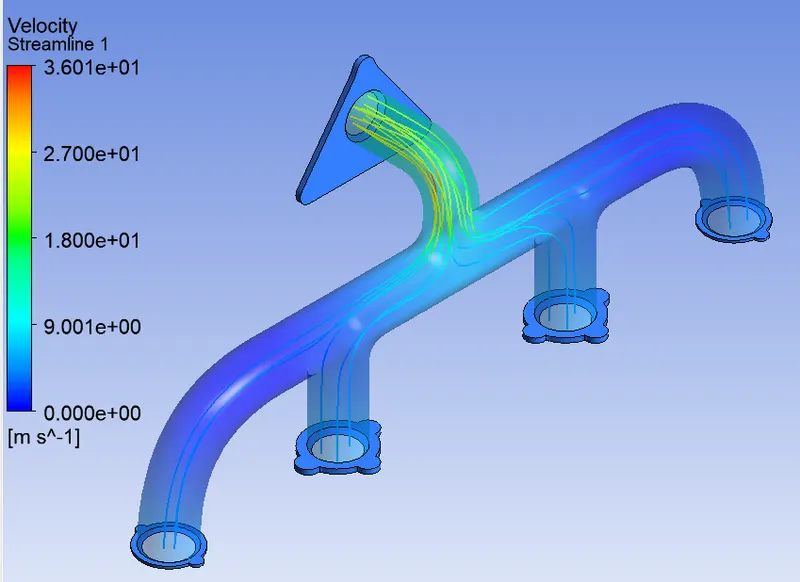
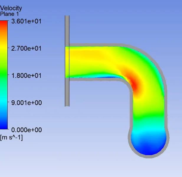
Velocity streamlines:

Temperature contour at outlet:

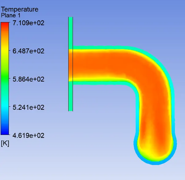
Velocity contour at outlet:

Surface heat transfer coefficient:

Velocity animation:

Analytical solution:

The reynolds number is 58189 which is turbulent, we use emperical relation between Nusselt,Reynolds & Prandtl numbers to find the Nusslet number.

`Nu = 0.023*Re^(0.8)*Pr^(0.3)`

Where:

`Pr = (muC_p)/k`

`mu = 1.7894e-05 (kg)/(ms)`

`C_p = 1006.43 J/(KgK)`

`Pr = 0.744`

n = 0.3 is constant heat tranfer that takes place from fluid to solid

`Nu = 0.0223*58189.8960^0.8*0.744^0.3`

`Nu = 136.4827`

heat transfer coefficient (h) = `(Nu*k)/D`

where k = thermal conductivity of material = `0.0242 W/(mK)`

h = `19.42 W/(m^2k)`

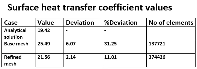
Heat transfer coefficient table comparing all cases:

Reason to select `komega-SST` model over `komega-epsilon` :

• `komega-epsilon` model is more suitable for finding values far away from the wall, where as `komega-SST` is more sutiable to calculate properties near to wall.
• Since we want to capture the heat transfer values at the interface and near to the wall `komega-SST` model is more suitable for our simulation.
• Since we are calculating properties in viscous sublayer where Y+ values vary from 1 to 5 `komega-SST` model is more suitable as it uses the Y+ values between 1-30.

Conclusion:

• CHT analysis of exhaust port is done using `komega-SST` model and using Y+ value of 1
• Deviation from the analytical solution is found to be 11%
• Velocity at the outlet is more then the inlet because we have 4 inlets from which fluid enters and only 1 outlet,since all the fluid that enters need to exit the outlet to satisfy continuity and mass conservation the velocity at the outlet is more compared to inlet.
• Temperature at the outlet is more than the inlet where hot fluids entering becasue of the increase in the velocity the turbulance increases this results in heat transfer to solid wall more compared to inlet where flow is less turbulent.