Week 4.1 - Genetic Algorithm

Genetic Algorithm:

Aim:–

To calculate the generic algorithm for calculating the local maxima and calculating the optimum values for a given function.

Introduction:–

Generic algorithm uses the method of random sampling. This method of solving constrained and unconstrained problems which are based upon selection. Generic algorithm is widely used to solve the optimization problems in different fields. Generic algorithm starts with an initial set of random solutions called Population. Each individual in the population is called chromosome representing a solution to the problem at hand. The chromosome evolves through the successive iterations, called generations. During each generation, the chromosomes are evaluated using some measures of fitness. To create a new generation, new chromosome are formed by either merging two chromosomes from current generation using a crossover operator or modifying a chromosome using mutation operator. A new generation is formed by selecting according to fitness values and rejecting others so as to keep the population size constant. Staligmite function is the mathematical model for generating the local minima and maxima.

Code for Staligmite function-

function[Z] = staligmite(input_vector)

x = input_vector(1);
y = input_vector(2);

f1x = (sin((5.1*(pi.*x))+0.5))^6;
f1y = (sin((5.1*(pi.*y))+0.5))^6;

f2x = exp((-4*log(2)).*((x-0.0667).^2/(0.64)));
f2y = exp((-4*log(2)).*((y-0.0667).^2/(0.64)));

%[Z] = (f1x.*f2x.*f1y.*f2y);

fx = -f1x.*f2x;
fy = f1y.*f2y;
[Z] = (fx.*fy);

end

Maxima is a function to represent the change of values from positive to negative. Hence, to find out the maxima of a given function, one of the value in the function[f(x)] is taken as negative. So that negative values of function minimum are obtained and the maxima can be determined. (i.e. Maxima = -Minima).

Main Code for GA-

clear all
close all
clc

x = linspace(0,0.6,100);
y = linspace(0,0.6,100);

n_var = 100;

[xx yy]= meshgrid(x,y);

for i= 1:length(xx)
    for j =1:length(yy)
        input_vector(1)=xx(i,j);
        input_vector(2)=yy(i,j);
        f(i,j) = staligmite(input_vector);
    end
end

 tic
for i = 1:n_var
    [input,fopt(i)] = ga(@staligmite,2);
        xopt(i) = input(1);
        yopt(i) = input(2);
end
studytime_case1 = toc

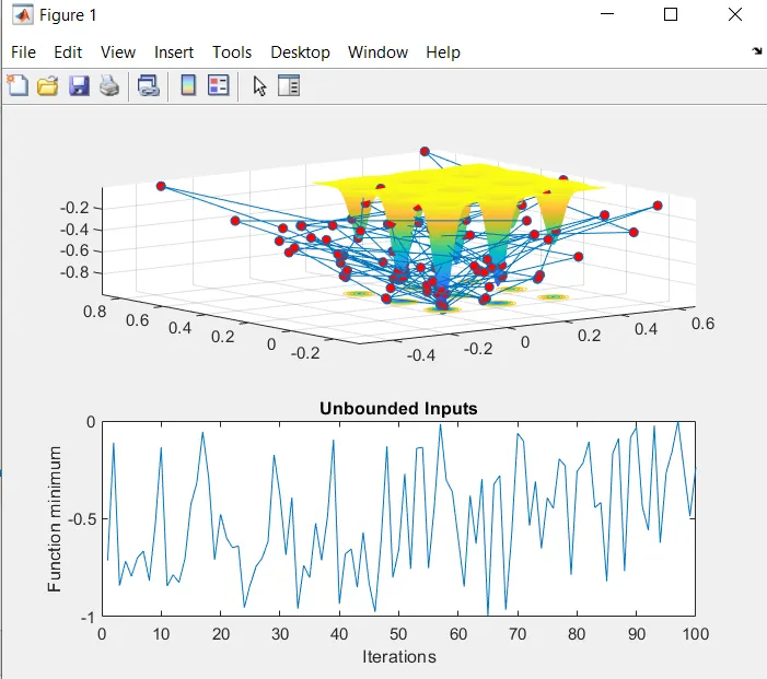
figure(1)
subplot(2,1,1)
surfc(x,y,f)
shading interp
hold on
plot3(xopt,yopt,fopt,'marker','o','markersize',5,'markerfacecolor','r')
subplot(2,1,2)
plot(fopt)
title('Unbounded Inputs');
xlabel('Iterations');
ylabel('Function minimum');

%Study case 2- Bounded inputs.
tic
for i = 1:n_var
    [input,fopt(i)] = ga(@staligmite,2,[],[],[],[],[0;0],[0.6;0.6]);
        xopt(i) = input(1);
        yopt(i) = input(2);
end
studytime_case2 = toc

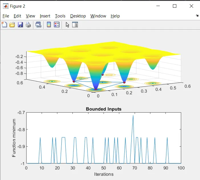
figure(2)
subplot(2,1,1)
surfc(x,y,f)
shading interp
hold on
plot3(xopt,yopt,fopt,'marker','o','markersize',5,'markerfacecolor','r')
subplot(2,1,2)
plot(fopt)
title('Bounded Inputs');
xlabel('Iterations');
ylabel('Function minimum');

%Study case 3- Bounded Inputs with Popolation size

options = optimoptions('ga');
options = optimoptions(options,'PopulationSize',500);

tic
for i = 1:n_var
    [input,fopt(i)] = ga(@staligmite,2,[],[],[],[],[0;0],[0.6;0.6],[],[],options);
        xopt(i) = input(1);
        yopt(i) = input(2);
end
studytime_case3 = toc

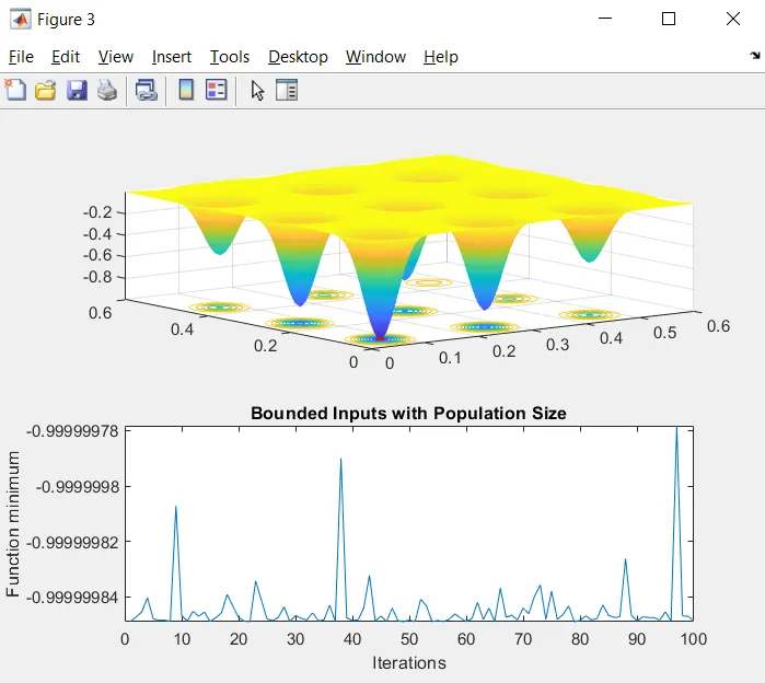
figure(3)
subplot(2,1,1)
surfc(x,y,f)
shading interp
hold on
plot3(xopt,yopt,fopt,'marker','o','markersize',5,'markerfacecolor','r')
subplot(2,1,2)
plot(fopt)
title('Bounded Inputs with Population Size');
xlabel('Iterations');
ylabel('Function minimum');   

Results-