Week 3 - Solving second order ODEs

AIM

To create a simple pendulum oscillation motion using a intode command (from scipy module) to solve a second-order differential equation.

Formulae used

`(d^2 θ)/〖dt〗^2 +b/m dθ/dt+g/l sinθ=0`

EXPLANATION

NOTE: we have to download the scipy module to perform this challenge.

Initially, we have to break down the 2^nd order equation into 1^st order for simplifying the equation because most of the solver solves only 1^st order equation. Initially, We have to code a function for the differential equation. Then coming to the main program we have to provide the essential parameter such as gravitational force, coefficient of damping ratio, etc. Then initial conditions, we have to define two conditions one is displacement and another one is velocity. We take initial velocity is 6m/s. initially, displacement is 0, as we know the pendulum starts from a theta as a starting point. A time limit of ten seconds with 500 iterations. Ode45 is I inbuilt command which solves an ordinary differential equation. Ode requires the function of the time span and the initial conditions to solve our problem. This function first integrates the values and solves the variable of our function by breaking down ie discretizing it. Then we have to plot all the rows of the 1^st column (DISPLACEMENT )as we have defined before. Then we have to plot all the rows of the 2^nd column (VELOCITY). The animate the pendulum by position in the string and bob. Defining the position is very important.use FOR loop to execute multiple values of theta. Use sin and cos function to the position(plotting each point) the point in the graph. For bob, we need to plot it exactly at the end of the string that is x1 and x2 in our main program. Then use the counter variable as an increment method to run them multiple times.

for animation, we need to save the photos in a separate folder. use command prompt to go to the file location and use magick command to stitch into a gif.

Animation link

https://drive.google.com/file/d/1dh7P2Y11J74oHL4e1L00UxvVkNCQklZt/view?usp=sharing

output graph

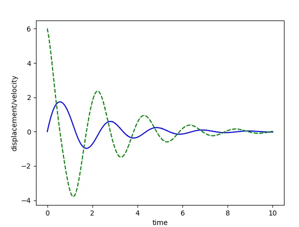
import math
import matplotlib.pyplot as plt 
from scipy.integrate import odeint
import numpy as np 




#function code
def model(theta,t,b,g,l,m):
	theta1 = theta[0]
	theta2 = theta[1]
	dtheta1_dt = theta2
	dtheta2_dt = -(b/m)*theta2 - (g/l)*math.sin(theta1)

	dtheta_dt=[dtheta1_dt,dtheta2_dt]
	return dtheta_dt


	

b=0.09#damping factor
g=9.81
l=1
m=0.1

theta_0=[0,6]

#time points
t=np.linspace(0,10,150)

#solving diffrential equation using ode
theta=odeint(model,theta_0,t,args=(b,g,l,m))


#plotresults

plt.plot(t,theta[:,0],'b-,')
plt.plot(t,theta[:,1],'g--,')

plt.xlabel('time')
plt.ylabel('displacement/velocity')
plt.show()

#plotting pendulum

displacement=theta[:,0]
ct=1

for i in displacement:
	theta1=i
	x0=0
	y0=0
	x1=l*math.sin(theta1)
	y1=-l*math.cos(theta1)
	ct=ct+1

	filename='test%05d.png' % ct

	plt.figure()

	plt.plot([x0,x1],[y0,y1])
	plt.plot([-2,2],[0,0,],linewidth=3)
	plt.plot(x1,y1,'o',markersize=25)
	plt.xlim([-1.5,1.5])
	plt.ylim([-1.5,0.25])
	plt.savefig(filename)

conclusion

Thus we have successfully animated the pendulum damping by solving the 2nd order differential equation.