Week 2 Air standard Cycle

Aim

To plot a PV graph for the otto cycle.

Formulae used

• `V_S = π/4 × d^2 × l`-Swept volume
• `V_C = V_S /((c r − 1 ))`-Clearance volume
• `P_2 = P_1 × ( ( c r )^γ )`
• `c = P _1 × ( ( V 1 ) ^γ )`

• `P _3 = P _2 × ( (T _3 )/ (T _2 ))`
• `P _4 = P _3 × ( (V_ 3)/ (V _4) ) ^γ`
• `t _2 = (P _2 × V _2 × T _1 )/( P _1 × V_1 )`

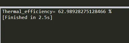
Thermal Efficiency output

Explanation

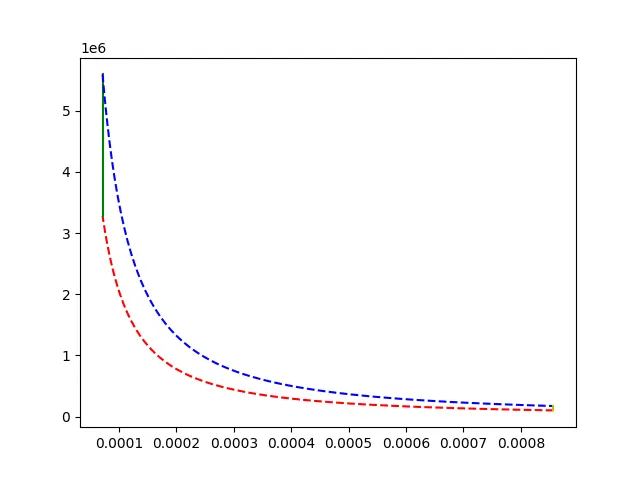
We need to plot the PV graph for the otto cycle. First, we need to predefine some standard parameters of the Engine like bore dia, stroke length, connecting rod length, and compression ratio. initial pressure P1 before compression and initial temperature T1 and max Temperature T3 is defined initially. We should also define the gamma which is used in PV relations. Using the relation pressure, temperature and volume we can easily plot the points of pressure and volume in the graph. But we know that the change in volume and pressure in the cylinder is not linear. So we use the function to identify the exact volume and pressure at the cylinder. We apply engine kinematics by using the formulae. To make it simple, we break down the formulae into three terms. This volume function will execute the volume at a particular function, say for example expansion or compression. Now we identified the volumes, to find the pressure we use pv=constant and we can run the program for each value of volume by just rearranging the formulae. Thus using plot commands we can plot the curves for volume and pressure .finally, we found the thermal efficiency using the formulae

output graph

• import math
  import matplotlib.pyplot as plt 
  import numpy as np
  
  
  
  def engine_kinematics(stroke,bore,cont_rod,cr,start_crank,end_crank):
  	a=stroke/2
  
  	R=cont_rod/a
  
  	vs=(math.pi/4)*pow(bore,2)*stroke
  	vc=vs/(cr-1)
  
  	sc = math.radians(start_crank)
  	ec = math.radians(end_crank)
  	
  
  	theta=np.linspace(sc,ec,100)
  
  	v=[]
  
  
  	for i in theta:
  		
  		term1= 0.5*(cr-1)
  		term2=R+ 1-math.cos(i)
  		term3=pow(R,2)-pow(math.sin(i),2)
  		term3=pow(term3,0.5)
  
  		v.append((1+term1*(term2-term3))*vc)
  	return v	
  		
  
  
  #engine geometric paramaeters
  stroke=0.1;
  bore=0.1;
  cont_rod=0.15;
  cr=12;
  
  #input 
  gamma=1.4
  t3=2300
  
  
  #state point 1 variables 
  
  p1=101325
  t1=500
  t3=2300
  
  #formulae for sept volume and clearance volume
  
  vol_swept=(math.pi/4)*pow(bore,2)*stroke
  
  vol_clr=vol_swept/(cr-1)
  
  
  v1=vol_swept+vol_clr
  
  v2=vol_clr
  #state point 2 variables
  #p2v2^gamma=p1v1^gamma
  #v1/v2 is nothing but cr
  
  p2=p1*pow(cr,gamma)
  
  
  
  
  
  #using relation between pressure,volume and temperature by ideal gas law 
  #p1v1/t1=p2v2/t2
  t2= (p2*v2*t1)/(p1*v1)
  
  v_compression=engine_kinematics(stroke,bore,cont_rod,cr,180,0) 
  
  constant = p1*pow(v1,gamma)
  
  p_compression=[]
   
  for v in v_compression:
  	p_compression.append(constant/pow(v,gamma))
  	
  	
  
  #state point 3 variables
  #At combustion w.k.t otto cycle is constant volume process
  
  v3=v2
  
  #relation between pressure ,volume and temperature
  #as v3=v2 ,it get cancelled 
  
  p3=(t3*p2)/t2
  
  v_expansion=engine_kinematics(stroke,bore,cont_rod,cr,0,180) 
  
  constant = p3*pow(v3,gamma)
  
  p_expansion=[]
   
  for v in v_expansion:
  	p_expansion.append(constant/pow(v,gamma))
  
  
  
  #state point 4 variables
  
  v4=v1
  
  p4=p3*pow((v3/v4),gamma)
  
  t4=(p4*v4*t3)/(p3*v3)
  
  plt.plot(v_compression,p_compression,'r--')
  plt.plot([v2,v3,],[p2,p3,],'g')
  
  plt.plot(v_expansion,p_expansion,'b--')
  plt.plot([v4,v1],[p4,p1],'y')
  
  plt.show()
  
  
  
  
  #thermal efficiency
  
  r=cr
  Thermal_efficiency =1-1/pow(r,(gamma-1))
  #thermal efficiancy in percentage
  Thermal_efficiency=Thermal_efficiency*100
  print('Thermal_efficiency=',Thermal_efficiency,'%')
  

Conclusion

Thus we have plotted a Pv graph for the otto cycle.