Week 5 - Curve fitting

1. What does popt and pcov mean? (Watch the video to get some context)

popt is an array where all the coefficient of the equation is generated with respect to the polynomial degree.

pcov is a 2D array that consists of the covariance of popt. Covariance gives the relation between two values, so here pcov gives the relation values between pop values.

2. What does np.array(temperature) do?

An array is a collection of items stored at contiguous memory locations. The idea is to store multiple items of the same type together. In python, the array command is stored in a module called numpy. in our challenge temperature is stored in form of an array with 3200 data.

3. What does the * in *popt mean?

popt is an array which consists of all the coefficient of equation generated based on the degree of the polynomial

*popt is the command which gives the same coefficient of the equation but it will multiply with e and give the output

5. What needs to be done in order to make the curve fit perfectly?

To make a curve fit perfect the estimates should be taken into account. The perfect fit is a fit where it should match the original curve and shouldn't have any matches with the original curve and shouldn't have any scaling and centering errors in that particular degree of the polynomial. The R^2 value must be equal to 1 and The sum of squares due to error(SSE) =0.

4.To write a code to perform the curve fit for the given specific heat and temperature data.

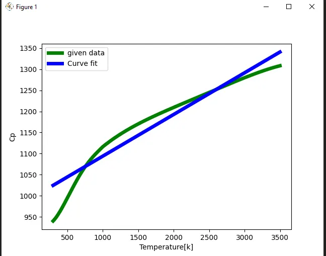
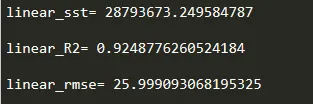
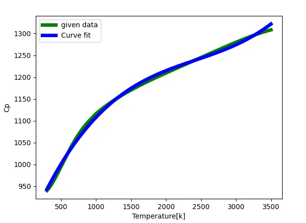
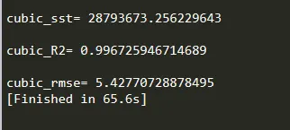
initially, we need to install a module called scipy where the curve fit command is pre-defined. then we need to define functions for the linear and cubic equations to perform the curve fit. next, we need the import the given data for specific heat(cp) and temperature and store it ina separate array. so we use the read and split command to split the data into two columns. To run multiple times we use for loop. after appending the cp and temperature in their respective array, we have to get popt and pcov by using a curve fit command (for linear /cubic both ).then we need to get the fit_cp value to compare it empirically. we need to check our fit how good its is so we use r^2 and rmse and sst method to check the error(for both linear and cubic equation to compare the fit with actual data)

FORMULAE USED

E – Error, SSE – Sum of squares due to errors, SSR- Sum of squares of regression,

SST – Total sum of squares, R2- R square, RMSE – Root mean square error, n – number of data.

`SSE=sum(E^2)`

`SSR=sum((P_(cp)-mean(cp))^2`

`SST=SSE+SSR`

`R2=(SSR)/(SST)`

`RMSE=sqrt((SSE)/n)

output for linear equation

error for linear equation

output for cubic equation

Error for cubic equation

import math
import matplotlib.pyplot as plt 
import numpy as np 
from scipy.optimize import curve_fit

def linear(t,a,b):
	return (t*a)+b

def cubic(t,a,b,c,d):
	return (a*pow(t,3)+(b*pow(t,2))+(c*t)+d)

def read_file():
	temperature=[]
	cp=[]
	for i in open('data','r'):
		line=i.split(',')
		temperature.append(float(line[0]))
		cp.append(float(line[1]))

	return [temperature,cp]

temperature,cp= read_file()
popt,pcov=curve_fit(linear,temperature,cp)



fit_cp=linear(np.array(temperature), *popt)

plt.figure(1)
plt.plot(temperature,cp,color="g",linewidth=5)
plt.plot(temperature,fit_cp,color="b",linewidth=5)
plt.legend(['given data','Curve fit'])
plt.xlabel('Temperature[k]')
plt.ylabel('Cp')
plt.show()


temperature,cp= read_file()
popt,pcov=curve_fit(cubic,temperature,cp)
fit_cp_1=cubic(np.array(temperature), *popt)

plt.figure(2)
plt.plot(temperature,cp,color="g",linewidth=5)
plt.plot(temperature,fit_cp_1,color="b",linewidth=5)
plt.legend(['given data','Curve fit'])
plt.xlabel('Temperature[k]')
plt.ylabel('Cp')
plt.show()

s=np.sum(cp)
l=np.size(cp)
m=s/l
print()
print('Mean of all cp:',m)

linear_sse=0
linear_ssr=0
for j in range(3200):
	linear_error=abs((np.sum((cp[j]-fit_cp[j]))))
	linear_sse=linear_sse+pow(linear_error,2)
	linear_ssr=linear_ssr+np.sum(pow((fit_cp[j]-m),2))
linear_sst= linear_ssr+linear_sse
linear_R2=linear_ssr/linear_sst
linear_rmse=pow((linear_sse/l),0.5)
print()

print('linear_sst=',linear_sst)
print()
print('linear_R2=',linear_R2)
print()
print('linear_rmse=',linear_rmse)

cubic_sse=0
cubic_ssr=0
for k in range(3200):
	cubic_error=abs((np.sum((cp[k]-fit_cp_1[k]))))
	cubic_sse=cubic_sse+pow(cubic_error,2)
	cubic_ssr=cubic_ssr+np.sum(pow((fit_cp_1[k]-m),2))
cubic_sst= cubic_ssr+cubic_sse
cubic_R2=cubic_ssr/cubic_sst
cubic_rmse=pow((cubic_sse/l),0.5)

print()
print('cubic_sst=',cubic_sst)
print()
print('cubic_R2=',cubic_R2)
print()
print('cubic_rmse=',cubic_rmse)

print("the value popt=",popt)
print("the value popt=",*popt)

CONCLUSION: So we can clearly conclude that the cubic polynomial equation gives a better result than the linear equation by the variation in the error.